7.2.4. Nonlinear Regression
7.2.4.0. Overview
The Nonlinear Regression procedure provides a least-squares method of fitting a user-specified function to a suitable data set. This regression function would usually be based on a theoretical model of the system under analysis, and can be written in terms of any number of independent variables and any number of parameters (subject to program restrictions). The user provides initial estimates for the parameter values, and the program then adjusts these over a number of iterations in order to obtain the best fit to the data (that is, minimise the residual sum of squares). The program ends by displaying a large number of output options regarding the parameters and fitted curve.
In addition to providing numerical values for the parameters and some related statistics, Nonlinear Regression can also be used to compare regression models. For example, with data describing an exponential decay curve, it is possible to assess (in a statistical sense) if the curve is monophasic:
![]()
or biphasic:
![]()
The same method can be used to compare two or more sets of data and determine if differences exist between them. This is explained in detail later in this section. First we shall look at the dialogues and facilities of this procedure.
7.2.4.1. Nonlinear Regression Variable Selection
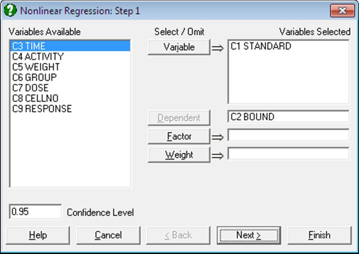
Dependent: Selection of a dependent variable containing numeric data is compulsory. Only one dependent variable can be selected.
Variable: At least one independent variable must be selected. It is not necessary for all independent variable columns selected in the Variables Selected list to be used in the analysis. The regression function is written as an expression involving variables C1, C2, … or their labels, and parameters P(1), P(2), … or their labels. Therefore, which columns are used depends on how the regression function is constructed.
Weight: A column of spreadsheet containing numeric data can be selected as weights. Cases with the highest weight value have the greatest effect on the fitted curve and those with the lowest weight have the least effect. If a weight variable is specified, then all entries in that data column must be greater than zero and not greater than 1.0E+10.
Factor: If a factor column is selected, the program can fit two or more curves simultaneously on the subgroups defined by the levels of the factor. This is useful when making comparisons between sets of data. The program can deal with up to eight curves, using the first eight levels of a factor.
7.2.4.2. Nonlinear Regression Setup Dialogue
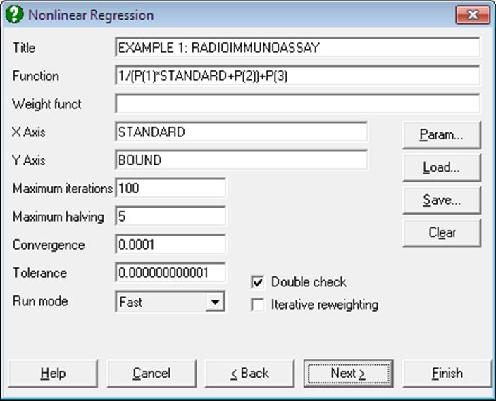
This dialogue allows you to enter all the information needed to specify how the regression is to be performed. All this information can be saved in a Nonlinear Regression setup file and loaded back when needed, which makes repeating the same or similar analyses on several data files much easier.
7.2.4.2.1. Buttons
The four buttons provided have the following tasks:
Param: Shortened for parameters. It will activate the Parameter Setup Dialogue.
Load: This will invoke the standard windows dialogue for opening a file. You can load a previously saved Nonlinear Regression setup file. The default extension is .USN.
The names and column numbers of all variables selected from the spreadsheet (dependent variable, all independent variables and if any, weight and factor variables) are recorded in the setup file. When the setup file is subsequently loaded, these will be checked against the actual selections made from the Variable Selection Dialogue so that there are no inconsistencies between the setup file and the variables in the spreadsheet. If there are inconsistencies, these will be reported, but it will still be possible to run an analysis. In this case, the selections made from the Variable Selection Dialogue will override the definitions in the setup file and it will be up to you to ensure that the variables used in various functions do refer to the correct columns in the spreadsheet.
Save: All current selections made in the Setup and Parameter dialogues, as well as the variable assignments made in the Variable Selection Dialogue will be saved in a binary file. The default extension is .USN and you are strongly recommended to keep that unchanged.
The [Save] option always saves the current values of parameters. Therefore, if this option is selected after the convergence has been achieved then the file may be saved with convergence parameters. Or more importantly, for particularly difficult problems, after breaking the run after a number of iterations, the current values of the parameters can be saved in the setup file making it possible to continue to run the model subsequently from where you left.
Clear: This will clear all controls in both Setup and Parameter dialogues for a fresh restart.
7.2.4.2.2. Controls
Title: This is a line of text you may enter to annotate a particular Nonlinear Regression setup and will also be printed as a sub title (after the procedure name) in the output.
Function: The regression function is entered as an expression involving the independent variable(s) and parameters. The independent variables are referred to with their labels or column numbers (C1, C2, etc.), and the parameters as P(1), P(2), etc.
As an example, to fit an exponential decay curve with the independent variable in C1, the function can be written as:
P(1)*Exp(C1*P(2))
If C1 has a label TIME and parameters 1 and 2 named ACTIVITY0 and RATE respectively, then the expression can be written as:
ACTIVITY0*Exp(TIME*RATE)
Weighting Function: Iterative reweighting can be used, which means that at each iteration the weights to be used in that iteration are calculated according to an expression (the weighting function) which is supplied by the user. This function is written in the same way as the regression function, except that a variable containing the fitted values V(0) can also be used.
The weight values generated in this way must be greater than zero and not greater than 1.0E+10, otherwise an error will be generated. The weighting function will only be used if the iterative reweighting option (see below) is enabled.
If a weights variable has been selected and iterative reweighting enabled, then an error will be reported. They cannot be used at the same time.
X-Axis: A transform expression for the horizontal axis of the graphical display must be entered. In the simplest case this will be a single variable (e.g. TIME or C1 for the example described above), but any expression containing more than one independent variable can be used. This expression must not include parameters or the dependent variable.
Y-Axis: As above but applies to the vertical axis of the graphical display. The dependent variable must be included in the Y-axis expression.
Max Iterations: This is the maximum number of iterations to be performed (default value is 100). It is seldom necessary to alter this value, since the program will terminate when the best fit has been obtained and the residual sum of squares stops changing from one iteration to the next (see Converge below). Also, the program can be interrupted at any time. Setting the maximum number of iterations to zero has the same effect as selecting Run Mode = FINISH (see below). A negative value will cause an error to be reported.
Max Halving: At each iteration the program calculates a correction vector for each active parameter which is used to modify that parameter value. The new parameter values generated will usually result in a decrease in the residual sum of squares (RSS), but if the RSS increases then the correction vectors are halved and their signs reversed (subject to lower/upper limits on the parameters) until a decrease in the RSS is obtained or the maximum number of step halving has been performed. The default value is five and the minimum is zero. A negative value will cause an error to be reported. The setting for Max Halving is only relevant if Run Mode = STANDARD (see below).
Converge: The program will terminate when the absolute fractional change in the RSS over three successive iterations is less than the value specified for Converge. The default value is 0.0001, meaning that if the RSS changes by less than 0.01% over three iterations then it is assumed that the best fit (minimum RSS) has been obtained. The final calculations are made and the results are then displayed.
Tolerance: The pivoting tolerance value should not normally be changed from its default value of 1.0E-11. However, when fitting a function which is more complex (has more parameters) than necessary the program may become unstable, evidenced by the RSS increasing rather than decreasing. This does not immediately indicate a program failure, but if it persists for 10 iterations or more, then some corrective action will probably be needed. This can usually be accomplished by specifying different initial estimates and / or supplying appropriate lower / upper limits for the parameters. If the instability is still present then increasing the tolerance value to 1.0E-5 may be helpful.
Run Mode: This determines how the program operates. The four options available are:
1) FAST: The regression is performed using the Marquardt-Levenburg algorithm, which in most cases is much faster than the conventional Gauss-Newton method. However, the Marquardt-Levenburg method as implemented in this program is less suitable for difficult regression analyses and will fail if there is an excessively high correlation between two or more parameters. If this happens the program will automatically switch to STANDARD mode. Difficult regression analyses may include those in which a) for certain combinations of parameter values, a large change in RSS accompanies a very small change in the value(s) of one or more parameters; b) an inappropriate regression model has been specified, which might be done intentionally in order to compare it statistically with another model; and c) there is excessive correlation between the parameters.
2) STANDARD: The regression is performed using a slower but much more stable method based on the conventional Gauss-Newton algorithm, which can cope with difficult analyses as described above. Since the program will change from FAST to STANDARD mode itself when needed, it is not necessary to start in this mode. However, if an inappropriate regression model (particularly one that is more complex or has more parameters than necessary) is being used, then beginning the analysis in STANDARD mode may give somewhat different parameter values; the extra parameters tend not to change from their initial values in this mode.
3) FINISH: The final calculations are made on the current parameter values and the results are displayed. These statistics (the parameter standard errors, correlation matrix and predicted standard deviations of the fitted curve) are only valid if a good fit to the data has been obtained.
4) MANUAL: In this mode the user enters a set of parameter values and the program then shows the corresponding fitted curve and RSS. This process repeats until the user exits from this part of the program. The program does not alter the parameter values, except for evaluation of any parameter constraint expressions that have been defined. If weighting or iterative reweighting has been enabled then the weighted RSS is calculated. This mode can be used to obtain initial parameter estimates for the regression, or to examine the effect of changing the parameter values on the fitted curve.
Double Check: If the regression converges in FAST mode and the fitted curve satisfies a built-in goodness-of-fit test (see 7.2.4.6. Technical Details) then the final calculations are made and the results displayed. If the fitted curve fails the goodness-of-fit test then the STANDARD mode is entered automatically. However, if Double Check is enabled then the program will switch to STANDARD mode to see if any further improvement in fit can be obtained (which does sometimes happen). The default settings (Run Mode = FAST and Double Check = On) are recommended for most applications.
Iterative Reweighting: this enables iterative reweighting as explained above for weighting function.
7.2.4.2.3. Parameter Setup Dialogue
The program will determine the number of parameters used in the regression from the number of rows filled in by the user. The minimum is one and the maximum is fifty.
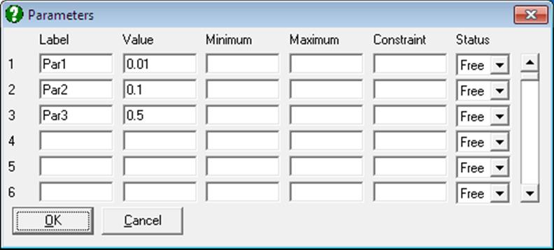
Label: These are optional, and can be used instead of the parameter numbers P(1), P(2), etc.
Value: In Nonlinear Regression the user must specify an initial value for each parameter which the program will then adjust in order to minimise the residual sum of squares. These initial estimates should be close to the true (or best-fit) values, but exactly how close they need to be depends on various factors such as the amount or error in the data and the complexity of the regression function. The initial values might be determined from the theory underlying the Regression Analysis, prior knowledge of the system, or graphical examination of the data.
The initial parameter values may be set to zero, but this will slow the program down quite markedly. A blank field does not have a zero value.
On completion of the Regression Analysis, the final parameter values are written back to the Parameter Setup Dialogue where they can be edited if necessary and used as starting values for further analysis.
Minimum: This is the minimum value that each parameter can take during the regression. A blank field means that no lower limit is imposed.
Maximum: This sets the maximum value for each parameter.
Although optional, it is recommended that lower and upper limits should be assigned for each parameter as a precaution against arithmetic errors. For example, if the regression function includes the square root of a parameter, then that parameter should have a lower limit of zero. Also, if the theory underlying Regression Analysis indicates that some parameter could not have a negative value, then that parameter would also have a lower limit of zero. Otherwise, quite broad limits can be set; parameters should not be restricted to a very narrow range unless there is special reason to do so.
If lower and / or upper limits have been set, then the initial value must be within the defined range otherwise an error will be reported when the Regression Analysis is started.
Constraint: This is the constraint expression referred to above. The expression is written in terms of other parameters only and must not include any of the input variables. The constraint expression will only be used if the corresponding parameter status is set to Constrained.
Status: This control determines how the parameter will be handled during the regression. There are three possible values:
1) Free: The value of the parameter will be adjusted in an attempt to obtain the best fit.
2) Fixed: The parameter value is fixed (constant) and it will not change.
3) Constrained: The value of the parameter is determined by other parameter values according to an expression (a parameter constraint expression) which you must supply. For example, if you wanted to perform the regression such that parameter 5 always had the same value as parameter 3, then parameter 5 would have status Constrained and the constraint expression should be P(3). If a parameter has status Constrained then the corresponding parameter constraint expression must be defined.
Parameters with status Free are termed active parameters. There must be at least one active parameter, otherwise an error will be reported.
7.2.4.3. Running the Program
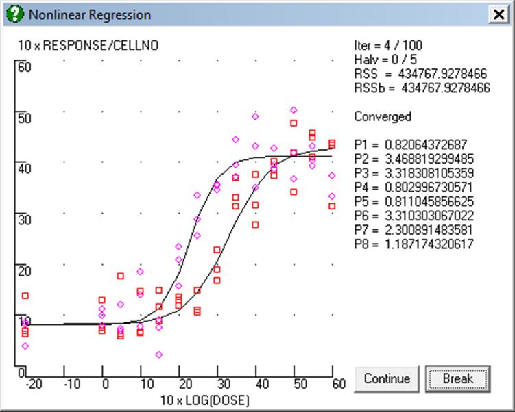
After filling in the Nonlinear Regression Setup Dialogue and the Parameter Setup Dialogue, click [Next] to run the model. The program will first check all the entries and report any inconsistencies found. Otherwise a new window is opened showing a bivariate plot of data according to the X-axis and Y-axis expressions defined in the Nonlinear Regression Setup Dialogue. At each iteration, the progress of fitting can be followed visually. The same window will also display the current values of number of iterations, residual sum of squares, as well as the current values of the parameters.
It is possible to interrupt or break the program while it is running by pressing <Escape>. However, the response may not be immediate, as the program will always finish the current iteration before stopping. When this happens, the Nonlinear Regression Setup Dialogue will be displayed. The current values can be saved to a regression setup file to continue later on, or change some of the parameters manually. When [Continue] is clicked, the program will resume iterations. Changing the regression function will result in a complete resetting of the regression run.
If the iterations continue with no sign of convergence, you may break the run, select the FINISH mode from the Nonlinear Regression Setup Dialogue and force the program to perform calculations necessary for output options.
7.2.4.4. Nonlinear Regression Output Options
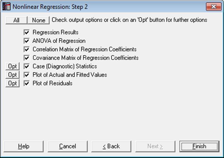
After convergence has been achieved or the program is stopped before convergence and Run Mode = FINISH has been selected, the Output Options Dialogue will be displayed. For a sample printout of the full Nonlinear Regression output (see 7.2.4.5. Nonlinear Regression Examples).
The Actual and Fitted Values, Residuals, Confidence Intervals for Actual Y Values and Interpolation options that existed in earlier version of UNISTAT are now combined under the Case (Diagnostic) Statistics option.
Regression Results: The main regression results include a report on whether the convergence has been achieved and the result of a goodness-of-fit test, which will be either OK or Failed test.
All values related to parameters are displayed in a table. These include minimum, maximum, coefficient estimate, standard error and status (Free, Fixed or Constrained). Confidence intervals for regression coefficients are also displayed for the user-defined confidence level. The entire table can be sent to the spreadsheet for further analysis.
Statistics reported include residual sum of squares, root mean square error, number of parameters, number of active parameters, number of cases, degrees of freedom (number of cases minus number of active parameters), R-squared and Durbin-Watson statistic.
Standard errors are only available for parameters with status Free. If a factor column has been selected, then most of the statistics will be displayed for each sub group separately.
ANOVA of Regression: The ANOVA table compares the regression model with the null hypothesis that “Y = constant”.
Correlation Matrix of Regression Coefficients: Only parameters with status Free are included in this table.
Covariance Matrix of Regression Coefficients: Only parameters with status Free are included in this table.
Case (Diagnostic) Statistics:
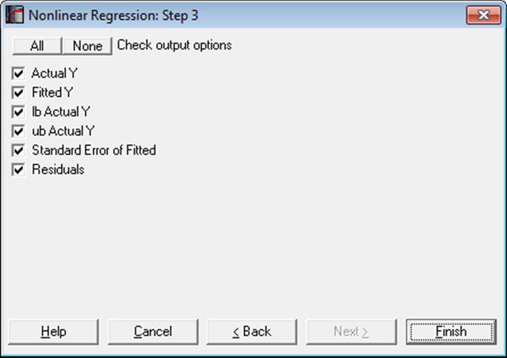
Predictions (Interpolations): As of this version of UNISTAT, the Interpolation output option is removed and the predicted Y values can be generated as in Linear Regression (see 7.2.1.2.2. Linear Regression Case Output). If, for a case, all independent variables are non-missing, but only the dependent variable is missing, a value will be predicted for the fitted Y value from the estimated regression equation. When a case is predicted, its label will be prefixed by an asterisk (*).
Statistics available under Case (Diagnostic) Statistics option are as follows.
Actual Y: Observed values of the dependent variable.
![]()
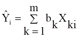
Fitted Y: Estimated values of the dependent variable.
Confidence Intervals for Actual Y-values: Confidence intervals for actual Y values are displayed. The default confidence level is 95%, but any value can be entered from the Variable Selection Dialogue.
![]()
Where ![]() is the critical value from the
t-distribution for an α / 2 level of significance and 1 degree of
freedom.
is the critical value from the
t-distribution for an α / 2 level of significance and 1 degree of
freedom.
Standard Error of Fitted:
![]()
Residuals:
![]()
Plot of Actual and Fitted Values: Actual and fitted Y values, as well as their confidence intervals, are plotted. The X-axis variable is as selected in the Nonlinear Regression Setup Dialogue.
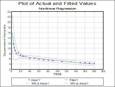
As with plots in Linear Regression and Polynomial Regression, the data points here are also interactive, but pressing <Delete> when a point is highlighted will not omit this point and re-run the analysis.
Plot of Residuals: A scatter plot of residuals is drawn against the dependent variable.
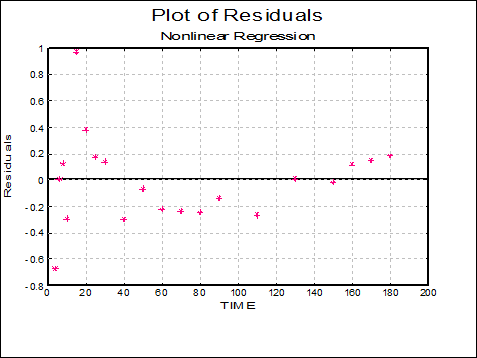
7.2.4.5. Nonlinear Regression Examples
7.2.4.5.1. Example 1: Radioimmunoassay
This is a simple example based on a calibration curve for a type of assay. Open NONLINRG and select Statistics 1 → Regression Analysis → Nonlinear Regression. The data consists of 14 cases and two variables STANDARD and BOUND.
Select STANDARD (C1) as the independent variable by clicking [Variable], and BOUND (C2) as the [Dependent] variable. Then clicking [Next], the Nonlinear Regression Setup Dialogue will be opened. Click on the [Load] button and load the NONLIN1.USN setup file. The function involves three parameters:
![]()
which is entered as:
1/((P(1)*STANDARD+P(2))+P(3)
or could be entered as:
1/((P(1)*V(1)+P(2))+P(3)
The three parameters have initial values of 0.01, 0.1 and 0.1 respectively, all have status Free, and no lower or upper limits are set. With the default settings of Run Mode = FAST and Double Check = On, the program converges after 8 iterations, then switches to STANDARD mode and performs another 3 iterations, at which point it converges again. The following are the main results:
Nonlinear Regression
Regression Results
EXAMPLE 1: RADIOIMMUNOASSAY
BOUND = 1/(P(1)*STANDARD+P(2))+P(3)
Convergence achieved at iteration 11, No of halving = 0
Goodness of Fit: OK
|
Parameter |
Minimum |
Maximum |
Estimate |
Standard Error |
Status |
Lower 95% |
Upper 95% |
|
Par1 |
|
|
0.0279 |
0.0019 |
Free |
0.0237 |
0.0321 |
|
Par2 |
|
|
1.0914 |
0.0171 |
Free |
1.0538 |
1.1291 |
|
Par3 |
|
|
0.0160 |
0.0153 |
Free |
-0.0177 |
0.0496 |
|
Residual Sum of Squares = |
0.0018 |
|
Root Mean Square Error = |
0.0126 |
|
Number of Parameters = |
3 |
|
No of Active Parameters = |
3 |
|
Number of Cases = |
14 |
|
Degrees of Freedom = |
11 |
|
R-squared = |
0.9983 |
|
Durbin-Watson Statistic = |
2.5336 |
ANOVA of Regression
|
Due To |
Sum of Squares |
DoF |
Mean Square |
F-Stat |
Prob |
|
Regression |
1.005 |
2 |
0.503 |
3141.719 |
0.0000 |
|
Error |
0.002 |
11 |
0.000 |
|
|
|
Total |
1.007 |
13 |
0.077 |
|
|
Correlation Matrix of Regression Coefficients
|
|
1 |
2 |
3 |
|
1 |
1.0000 |
0.7328 |
0.9336 |
|
2 |
0.7328 |
1.0000 |
0.8761 |
|
3 |
0.9336 |
0.8761 |
1.0000 |
Covariance Matrix of Regression Coefficients
|
|
1 |
2 |
3 |
|
1 |
0.0000 |
0.0000 |
0.0000 |
|
2 |
0.0000 |
0.0003 |
0.0002 |
|
3 |
0.0000 |
0.0002 |
0.0002 |
Case (Diagnostic) Statistics
|
|
Actual Y |
Fitted Y |
95% lb Actual Y |
95% ub Actual Y |
Standard Error of Fitted |
Residuals |
|
1 |
0.9472 |
0.9322 |
0.8638 |
1.0006 |
0.0054 |
0.0150 |
|
2 |
0.9255 |
0.9322 |
0.8638 |
1.0006 |
0.0054 |
-0.0067 |
|
3 |
0.8201 |
0.8284 |
0.7637 |
0.8930 |
0.0051 |
-0.0083 |
|
4 |
0.8312 |
0.8284 |
0.7637 |
0.8930 |
0.0051 |
0.0028 |
|
5 |
0.7254 |
0.7457 |
0.6742 |
0.8172 |
0.0056 |
-0.0203 |
|
6 |
0.7530 |
0.7457 |
0.6742 |
0.8172 |
0.0056 |
0.0073 |
|
7 |
0.5679 |
0.5750 |
0.4885 |
0.6614 |
0.0068 |
-0.0071 |
|
8 |
0.5910 |
0.5750 |
0.4885 |
0.6614 |
0.0068 |
0.0160 |
|
9 |
0.4324 |
0.4181 |
0.3315 |
0.5048 |
0.0068 |
0.0143 |
|
10 |
0.4105 |
0.4181 |
0.3315 |
0.5048 |
0.0068 |
-0.0076 |
|
11 |
0.2782 |
0.2736 |
0.2024 |
0.3448 |
0.0056 |
0.0046 |
|
12 |
0.2634 |
0.2736 |
0.2024 |
0.3448 |
0.0056 |
-0.0102 |
|
13 |
0.1772 |
0.1659 |
0.1161 |
0.2156 |
0.0039 |
0.0113 |
|
14 |
0.1546 |
0.1659 |
0.1161 |
0.2156 |
0.0039 |
-0.0113 |
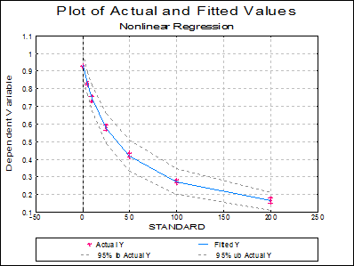
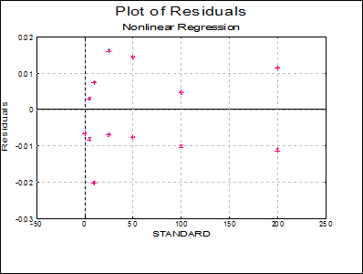
7.2.4.5.2. Example 2: Biphasic Exponential Decay
This example will illustrate the comparison of regression models. Open NONLINRG and select Statistics 1 → Regression Analysis → Nonlinear Regression. The data for this example consists of 21 cases and 3 variables.
Select TIME (C3) as the independent [Variable], ACTIVITY (C4) as the [Dependent] variable, and WEIGHT (C5) as the [Weight] variable. Click [OK] and after the Nonlinear Regression Setup Dialogue is displayed click on the [Load] button and load the NONLIN2.USN setup file.
The function involves 4 parameters (INIT1, RATE1, INIT2, RATE2) and describes the following biphasic exponential decay curve:
ACTIVITY = INIT1*Exp(RATE1*TIME)+INIT2*Exp(RATE2*TIME)
which could be entered, without variable or parameter names, as
P(1)*Exp(P(2)*C1)+P(3)*Exp(P(4)*C1)
The parameters have initial values of 10, -0.1, 5 and -0.01 respectively, all have status Free, and no lower or upper limits are set. The program will perform 8 iterations in FAST mode, then 3 iterations in STANDARD mode, and then the results are displayed.
Nonlinear Regression
Regression Results
EXAMPLE 2: BIPHASIC EXPONENTIAL DECAY
ACTIVITY = INIT1*EXP(RATE1*TIME)+INIT2*EXP(RATE2*TIME)
Convergence achieved at iteration 11, No of halving = 0
Goodness of Fit: OK
|
Parameter |
Minimum |
Maximum |
Estimate |
Standard Error |
Status |
Lower 95% |
Upper 95% |
|
INIT1 |
|
|
14.0304 |
1.5996 |
Free |
10.6554 |
17.4054 |
|
RATE1 |
|
|
-0.2627 |
0.0320 |
Free |
-0.3303 |
-0.1952 |
|
INIT2 |
|
|
7.4943 |
0.1836 |
Free |
7.1071 |
7.8816 |
|
RATE2 |
|
|
-0.0034 |
0.0002 |
Free |
-0.0039 |
-0.0029 |
|
With normalised weights: |
|
|
Residual Sum of Squares = |
1.4317 |
|
Root Mean Square Error = |
0.2902 |
|
With absolute weights: |
|
|
Residual Sum of Squares = |
40.0617 |
|
Root Mean Square Error = |
1.5351 |
|
Number of Parameters = |
4 |
|
No of Active Parameters = |
4 |
|
Number of Cases = |
21 |
|
Degrees of Freedom = |
17 |
|
R-squared = |
0.9863 |
|
Durbin-Watson Statistic = |
0.8836 |
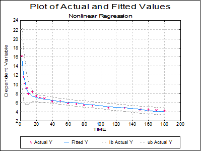
The rest of the output options are not reproduced here.
The output is essentially the same as for Example 1, except for weights. When weights are used, two RSS values are shown; the first is obtained with a normalised set of weights used for internal calculations and the second with the absolute weight values from the data file (or those calculated using the weighting function). The normalised weights have a mean value of 1.0 and are proportional to the absolute values. Since the RMS error is obtained from the RSS, there are also two entries for RMSerror. If the weights only indicate reliability of each data point relative to the others, it would be more appropriate to use the normalised RSS for reporting purposes or further calculations.
Although the fitted curve passes the goodness-of-fit test, the graphical display (plot of ACTIVITY against TIME) might suggest a slight systematic deviation of the data points about the curve. Interpretation of this would depend on the theoretical basis for the analysis, but suppose that a six parameter model was considered possible:
ACTIVITY = INIT1*Exp(RATE1*TIME)+INIT2
*Exp(RATE2*TIME)+INIT3*Exp(RATE3*TIME)
To establish if there is any statistical basis for accepting the six parameter model in preference to the four-parameter model, it is necessary to perform the regression again using the more complex function and then compare both sets of results on the basis of change in RSS with change in number of degrees of freedom for the regression using an extra-sum-of-squares test (sometimes referred to as an F-ratio test).
Altering the regression setup is quite simple: assign labels and initial values to parameters 5 & 6 of INIT3 and RATE3 and 1.0 and -0.001 respectively, and include these parameters in the regression function as shown above. Also, assign a maximum value of zero for each RATE parameter. The regression can now be performed (taking about 60 iterations) using the six parameter model. The results will be as follows.
Nonlinear Regression
Regression results
EXAMPLE 2: BIPHASIC EXPONENTIAL DECAY
Convergence achieved at iteration 52, no of halving = 0
Goodness of Fit Test: OK
|
Parameter |
Minimum |
Maximum |
Estimate |
Std Error |
|
INIT1 |
|
|
16.8864 |
2.2845 |
|
RATE1 |
|
0 |
-0.4513 |
0.0806 |
|
INIT2 |
|
|
3.1163 |
0.5334 |
|
RATE2 |
|
0 |
-0.0438 |
0.0168 |
|
INIT3 |
|
|
6.4984 |
0.4217 |
|
RATE3 |
|
0 |
-0.0024 |
0.0004 |
|
With normalised weights: |
|
|
Residual Sum of Squares = |
0.4571 |
|
Root Mean Square Error = |
0.1746 |
|
With absolute weights: |
|
|
Residual Sum of Squares = |
12.7893 |
|
Root Mean Square Error = |
0.9234 |
|
Number of Parameters = |
6 |
|
No of Active Parameters = |
6 |
|
Number of Cases = |
21 |
|
Degrees of Freedom = |
15 |
|
R-squared = |
0.9338 |
|
Durbin-Watson statistic = |
2.0314 |
The null hypothesis is that “there is no difference in RSS between the two models”. The RSS has actually decreased by about 60%, but it is necessary to assign a significance level to this (the probability of rejecting the null hypothesis when it is true). For the following calculations it does not matter if the RSS values were obtained with normalised or absolute weights, except that you should use the same one throughout (normalised values are used below – this method is equally applicable to comparison of unweighted regression analyses). Defining;
Model 1 (4 parameters): RSS1 = 1.43174 with DF1 = 17
Model 2 (6 parameters): RSS2 = 0.45707 with DF2 = 15
an F-statistic is calculated as:
![]()
with (DF1 – DF2) and DF2 degrees of freedom.
This gives F = 15.993 with 2 & 15 degrees of freedom. From statistical tables the associated p-value is less than 0.001, and consequently the null hypothesis can be rejected. That is, the six-parameter model might be said to give a significantly better fit.
In fact, a five-parameter model:
ACTIVITY = INIT1*Exp(RATE1*TIME)+INIT2
*Exp(RATE2*TIME)+CONSTANT
results in a significant decrease in RSS compared with the four-parameter model (P < 0.001), but there is only a slight difference in RSS between this and the six-parameter model (P > 0.05). This five-parameter model can be specified either by rewriting the regression function in terms of five parameters, or using the six-parameter model with P(6) = 0 and with status Fixed (parameter 6 is held constant with a value of zero).
7.2.4.5.3. Example 3: Dose-Response Curves
This example will show how the program can be used to fit two (or more) curves simultaneously and to make comparisons between them using the F-ratio method.
Open NONLINRG and select Statistics 1 → Regression Analysis → Nonlinear Regression. The data for this example consists of 84 cases and 4 variables. Select GROUP (C6) as the Factor, DOSE (C7) and CELLNO (C8) as the independent [Variable]s and RESPONSE (C9) as the [Dependent] variable. Click [OK] to proceed and when the Nonlinear Regression Setup Dialogue is displayed click on the [Load] button and load NONLIN3.USN regression setup file.
Suppose that in a pharmacology experiment, batches of cells are grown, subjected to some treatment or left untreated as the controls, then exposed to different concentrations of a drug and the response of the cells to that drug measured. The purpose of the experiment is to determine if the treatment has any effect on the drug response and if so, to describe that effect. The dose-response curve is sigmoid and can be described by the logistic function:
![]()
where:
DS1=DOSE^SLOPE
ES1=ED50*SLOPE
DOSE represents the dose of the drug (an independent variable) and RESPONSE is the measured response (the dependent variable). The four parameters are BASAL (the minimum or resting response), ACTIVE (the activatible response or maximum rise above basal), ED50 (the concentration of drug giving half-maximal activation) and SLOPE (which describes the steepness of the increase in response). Actually, ED50 is the logarithm of the dose giving half-maximal activation; it is appropriate to estimate the logarithm of this parameter since it has a log-normal distribution (a plot of ACTIVITY against Log(DOSE) is symmetrical about the point DOSE = ED50).
Further, suppose that three experiments are performed, each involving a paired control and treated group. The cell preparation is homogeneous within each of the three experiments but can vary between experiments. The response is assumed to be proportional to the number of cells present, which is also measured (CELLNO, another independent variable). The function is now:
![]()
and therefore the parameters BASAL and ACTIVE represent the response per unit cell number.
Since the data file represents two curves (control and treated), it is necessary to indicate which cases belong to each curve. A data grouping variable (GROUP) is included in the data file with values of 1 (control) or 2 (treated). The order in which the data points appear in the file has no effect on the regression.
Since a four-parameter function is used to describe one dose-response curve and the data describes two such curves, the regression will involve eight parameters. These are named BASAL:1, ACTIVE:1, ED50:1, SLOPE:1 (for group 1), and BASAL:2, ACTIVE:2, ED50:2 and SLOPE:2 (for group 2). It is now necessary to write the regression function in such a way that the value of GROUP is used to select which parameters are used in evaluating the function. The function is written:
(P((GROUP-1)*4+1)+P((GROUP-1)*4+2)*
(DOSE^P((GROUP-1)*4+4)/10^(P((GROUP-1)*4+3)*
P((GROUP-1)*4+4)))/(1+DOSE^P((GROUP-1)*4+4)/
10^(P((GROUP-1)*4+3)*P((GROUP-1)*4+4))))*CELLNO
Factor variable GROUP is used to calculate the parameter subscripts. When GROUP = 1, the function is equivalent to:
(P(1)+P(2)*(DOSE^P(4)/10^(P(3)*P(4)))/
(1+DOSE^P(4)/10^(P(3)*P(4))))*CELLNO
and when GROUP = 2 it is equivalent to:
(P(5)+P(6)*(DOSE^P(8)/10^(P(7)*P(8)))/
(1+DOSE^P(8)/10^(P(7)*P(8))))*CELLNO
In the setup file, the following parameter constraints are defined but not enabled (initially all parameters have status Free);
BASAL:2 = BASAL:1
ACTIVE:2 = ACTIVE:1
ED50:2 = ED50:1
SLOPE:2 = SLOPE:1
These will be used later in making comparisons between the two curves.
Finally, the transforms for the graphical display are defined:
X-Axis = Log(DOSE)
Y-Axis = RESPONSE/CELLNO
The first regression analysis can now be performed. For the purposes of the following discussion, this model (8 active parameters) is model 1. The results are as follows:
Nonlinear Regression
Regression Results
EXAMPLE 3: DOSE-RESPONSE CURVES / MODEL 1
RESPONSE = (P((GROUP-1)*4+1)+P((GROUP-1)*4+2)*(DOSE^P((GROUP-1)*4+4)/10^(P((GROUP-1)*4+3)*P((GROUP-1)*4+4)))/(1+DOSE^P((GROUP-1)*4+4)/10^(P((GROUP-1)*4+3)*P((GROUP-1)*4+4))))*CELLNO
Convergence achieved at iteration 16, No of halving = 0
Goodness of Fit: OK
|
Parameter |
Minimum |
Maximum |
Estimate |
Standard Error |
Status |
Lower 95% |
Upper 95% |
|
BASAL:1 |
0.0000 |
10.0000 |
0.8215 |
0.1194 |
Free |
0.5837 |
1.0592 |
|
ACTIVE:1 |
0.0000 |
10.0000 |
3.4658 |
0.2280 |
Free |
3.0116 |
3.9200 |
|
ED50:1 |
1.0000 |
5.0000 |
3.3174 |
0.1232 |
Free |
3.0720 |
3.5629 |
|
SLOPE:1 |
0.1000 |
5.0000 |
0.8061 |
0.1659 |
Free |
0.4757 |
1.1365 |
|
BASAL:2 |
0.0000 |
10.0000 |
0.8111 |
0.1304 |
Free |
0.5515 |
1.0707 |
|
ACTIVE:2 |
0.0000 |
10.0000 |
3.3104 |
0.1772 |
Free |
2.9575 |
3.6632 |
|
ED50:2 |
1.0000 |
5.0000 |
2.3012 |
0.0923 |
Free |
2.1173 |
2.4851 |
|
SLOPE:2 |
0.1000 |
5.0000 |
1.1878 |
0.2613 |
Free |
0.6674 |
1.7083 |
|
Group |
No |
RSSQ(n/w) |
R-squared |
D-W stat |
Fit |
|
1 |
42 |
207905.2146 |
0.9795 |
1.9323 |
OK |
|
2 |
42 |
226867.9214 |
0.9826 |
1.9267 |
OK |
|
Residual Sum of Squares = |
434773.1359 |
|
Root Mean Square Error = |
75.6353 |
|
Number of Parameters = |
8 |
|
No of Active Parameters = |
8 |
|
Number of Cases = |
84 |
|
Degrees of Freedom = |
76 |
|
R-squared = |
0.9381 |
|
Durbin-Watson Statistic = |
1.9277 |
The rest of the output options are not reproduced here.
The output is largely as described previously except that a new list is included in the Regression Results for each data group; the number of cases, the RSS and the result of the goodness-of-fit test. If weighting has been used then the RSS values are calculated using normalised weights as explained above.
From the graphical display there appears to be little difference in basal or maximal (basal plus activatible) responses, but there does seem to be a difference in ED50 and perhaps also in slope since, between minimum and maximum responses, the two curves are not completely parallel. To make a preliminary comparison between the two curves, we can determine if the difference between parameter values exceeds two standard errors of the difference, which would suggest a significant difference. That is, for parameters having values Pa and Pb with standard errors Ea and Eb, if:
![]()
then a genuine difference is likely. Using this method, the only apparent difference is between parameters 3 (ED50:1) and 7 (ED50:2). However, the F-ratio test is more reliable, and should be used in preference as demonstrated below.
To test the null hypothesis that “there is no difference of any kind between control and treated groups” (model 2), all four constraints are enabled. This gives a model with four active parameters, and results in RSS = 801471.4 with DF = 80. The goodness-of fit test returns Fail both for the entire data set and for both groups, which certainly indicates that this model is not appropriate. To compare models 1 & 2, the F-statistic is calculated as:
![]()
with (80-76) and 76 degrees of freedom. This gives F = 16.025 with 4 & 76 degrees of freedom and a p-value of less than 0.001. Therefore the null hypothesis is rejected and a genuine difference between the curves is established.
The preliminary analysis suggested no difference in BASAL or ACTIVE parameters between control and treated groups. To test this properly, the constraints for parameters 5 and 6 are enabled (thus BASAL:2 = BASAL:1 and ACTIVE:2 = ACTIVE:1. This is model 3, and results in RSS = 438789.1 with DF = 79, and all goodness-of-fit tests are passed. Comparison of models 1 & 3 gives an F-statistic of 0.351 with 2 & 76 degrees of freedom, and a corresponding p-value of greater than 0.1. Thus the null hypothesis “no difference in BASAL or ACTIVE parameters” is not rejected.
With constraints BASAL:2 = BASAL:1, ACTIVE:2 = ACTIVE:1 and SLOPE:2 = SLOPE:1 (model 4), the RSS is 446337.8 with DF = 79. Comparison of this with model 1 gives F = 0.927 with 3 & 76 degrees of freedom and a p-value of greater than 0.1. The null hypothesis “no difference in BASAL, ACTIVE or SLOPE parameters” is not rejected. It is sometimes necessary to carry out the comparisons in a stepwise manner. For example, having established no difference in BASAL or ACTIVE parameters, models 3 & 4 could be compared to further establish no difference in SLOPE parameters (which would give F = 1.341 with 1 & 78 degrees of freedom and p > 0.1, which is similar to the comparison of models 1 & 4).
Finally, with the single constraint ED50:2 = ED50:1 (model 5, null hypothesis “no difference in ED50 parameters”), we obtain RSS = 660274.5 with DF = 77. Comparison of this with model 1 gives F = 39.421 with 1 & 76 degrees of freedom and a p-value of less than 0.001, and therefore the null hypothesis is rejected.
Thus the preliminary analysis was correct in that the only
difference between control and treated groups is a change in ED50. The null hypothesis for the experiment would be that there is no difference
between control and treated groups (model 2). Comparison of this with model 4
(difference in ED50 only) gives F = 62.857 with 1 & 79
degrees of freedom and a p-value of less than 0.001. Using the results obtained
with model 4, it can be stated that the treatment had no effect on BASAL,
ACTIVE or SLOPE parameters (0.835 ![]() 0.085,
3.319
0.085,
3.319 ![]() 0.129, and 1.044
0.129, and 1.044 ![]() 0.156 respectively, p > 0.1) but
reduced the ED50 from 3.253
0.156 respectively, p > 0.1) but
reduced the ED50 from 3.253 ![]() 0.091 to
2.322
0.091 to
2.322 ![]() 0.091 (P < 0.001 using
the F-value of 62.857).
0.091 (P < 0.001 using
the F-value of 62.857).
7.2.4.6. Technical Details
The program seeks the set of parameter values that minimise the residual sum of squares (RSS):
![]()
or:
![]()
if weighting is used, where Yobs and Ypred are the observed and predicted values of the dependent variable, w is the weight, and the summation is over all cases. The predicted value Ypred is obtained by evaluation of the regression function f(v, p), where v represents the set of independent variables and p the parameters.
The Gauss-Newton method is implemented in two forms. In both, the program obtains for each case the residual (z, = Yobs – Ypred), and for each case and each active parameter (pi) the partial derivative
![]()
Using the approximation:
![]()
where the summation is over all active parameters and qi represents a correction vector for each such parameter, solution of the set of linear equations so generated provides an estimate for each qi. These correction vectors are used to generate a new set of parameter values for use in the next iteration, and this process is repeated until a termination condition is satisfied.
The partial derivatives are obtained arithmetically by
evaluation of f(v, p) at parameter values p and p ![]() delta.
The delta value is computed for each parameter as follows:
delta.
The delta value is computed for each parameter as follows:
1) If p = 0, then delta starts at 1.0E-30 and increments in steps of 10 until a suitable change in RSS is obtained or delta = p/10 or a boundary constraint is met.
2) If p![]() 0, then
delta starts at p/1000 and increments in steps of Sqr(10) until a suitable
change in RSS is obtained or delta = p/Sqr(10) or a boundary
constraint is met.
0, then
delta starts at p/1000 and increments in steps of Sqr(10) until a suitable
change in RSS is obtained or delta = p/Sqr(10) or a boundary
constraint is met.
In FAST mode, the delta values are computed on entry and subsequently recomputed only for any parameter that changes sign. The partial derivatives are obtained at parameter values p and (p + delta) or (p – delta) depending on any boundary constraints. In STANDARD mode, the delta values are computed at each iteration and the partial derivatives are obtained at parameter values (p + delta) and (p – delta) subject to any boundary constraints. If a suitable change in RSS is not obtained then the parameter is omitted from the current iteration (in FAST mode the delta value will be recomputed at the next iteration).
In FAST mode, solution of the set of linear equations is achieved by a matrix inversion method incorporating the Marquardt-Levenburg procedure provided that excessive correlation between parameters is not detected. In the presence of such correlation or in STANDARD mode, a stepwise multivariate regression method is used with omission of parameters until any excessive correlation is removed.
The correction vectors obtained are used to update the parameter values; in STANDARD mode if a reduction in RSS is not achieved with the new set of parameter values then the correction vectors are halved and their signs reversed (subject to any boundary constraints) until a decrease in RSS is obtained or the maximum number of step halvings has been performed. At the end of each iteration, the RSS is compared with the recorded best-fit value and if necessary the best-fit value and associated parameter values are updated.
Parameters subject to an equality constraint are not included in the steps described above, but the constraints are evaluated at all stages where the parameter values are altered (e.g. in calculating the partial derivatives). The constraint expressions are evaluated in the order in which the parameters are numbered; therefore a constraint expression for parameter b should not use the result of constraint imposed on parameter a unless b > a.
Iteration continues until a) the maximum number of iterations has been performed, b) the convergence criterion is satisfied, c) the user interrupts the program, or an error occurs (termination conditions). Convergence is achieved when the absolute fractional change in RSS over 3 successive iterations is less than a user-specified value (Converge, default 0.0001). In a) or b), the parameters are reset to the recorded best-fit values. If convergence occurs in FAST mode and either the Double Check facility is enabled or the fitted curve fails the goodness-of-fit test, further iterations are performed in STANDARD mode until a termination condition occurs again. If termination conditions a) or b) are met in FAST mode, then the parameter standard errors, correlations and standard deviations of the y-predicted values are calculated using the partial derivatives obtained in the last iteration providing that the RSS in that iteration is within 1 ± Convergence of the best-fit value and the goodness-of-fit test is passed. Otherwise (or in STANDARD mode) the partial derivatives are recomputed after resetting the parameters to the best-fit values and before the parameter standard errors etc. are calculated.
Standard errors and correlations are not computed for parameters that have zero or negligible effect on the fitted curve, for which an excessive correlation is present, or which are held constant or are the subject of an equality constraint (status Fixed or Constrained).
The goodness-of-fit test consists of two parts; a) a Runs Test assuming a binomial distribution with p = 0.5 is applied to the signs of the residuals and fail registered
at α ≤ 0.005; and b) the weighted mean and standard deviation of the
residuals is calculated and Fail registered if
zero is out with the interval mean ![]() 2 x
standard deviations. The test always returns Fail
if the number of cases is less than five.
2 x
standard deviations. The test always returns Fail
if the number of cases is less than five.
For further reading see Ratkowski, D. A. (1983) and Wadsworth, H. M. (1990).
