9.3.7. Data Transformation
The standard Process Capability Analysis is one of many statistical procedures that assume normal distribution of data. When this cannot be assumed, either capability indices should be computed based on distributions other than normal, or the data should be transformed so that it conforms better to the normal distribution. This procedure provides two Data Transformation options; a family of Johnson transformations (see Kotz, S. and Johnson, N.L. 1993) and the Box-Cox Transformation (see Box, G. E. P. and Cox, D. R. 1964). These two methods are also available as Data Transformation options within the Process Capability Analysis procedure. You can also use the Box-Cox Regression procedure to transform a dependent variable when predictor (independent) variables exist.
The Variable Selection Dialogue is of the multisample type (see 6.0.4. Multisample Tests), allowing selection of multiple data and factor columns. All selected data is pooled and sorted to form one continuous variable before it is transformed.
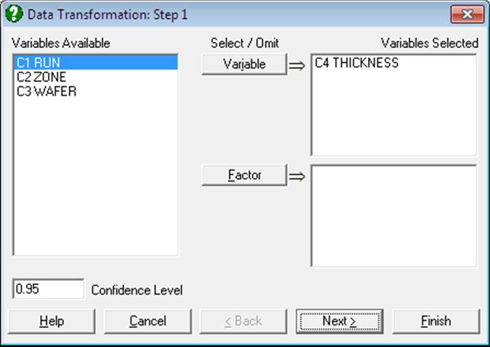
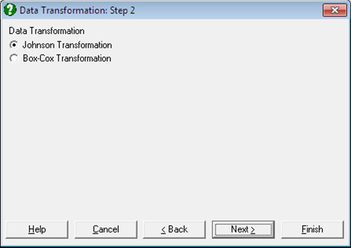
The next dialogue will ask for the type of transformation. Box-Cox Transformation will only work with positive data, whereas Johnson Transformation has no such restrictions. It must also be noted that in most cases Johnson Transformation is more powerful than Box-Cox Transformation and it will generate transformed variables more normally distributed.
9.3.7.1. Johnson Transformation
Johnson Transformation system consists of three types of curves:
Bounded system (SB):
![]()
Log-normal system (SL):
![]()
Unbounded system (SU):
![]()
where:
![]()
y is the transformed value
γ is the shape 1 parameter
η is the shape 2 parameter
ε is the location parameter
λ is the scale parameter.
The program evaluates all three functions with the current estimates of four parameters, transforms the data and runs a normality test on the transformed data. The four parameters are optimised until one of the three transformation functions produces the best normality test result. The algorithm is based on Polansky, A. M., Chou, Y.-M., and Mason, R. L., (1999), but the Shapiro-Wilk normality test is replaced with the more accurate Anderson-Darling Test.
Johnson Transformation may not always provide a solution. The best way to find out whether a solution has been found is to ensure that the transformed data produces a higher Anderson-Darling Test probability than the original data.
9.3.7.1.1. Johnson Transformation Output Options
Johnson Transformation Results:
Parameter estimates: The optimum levels for the four parameters are displayed.
Transformation Selected: The selected Johnson function is displayed together with constraints on parameters. The same equation is also printed on a separate line with estimated parameter values, in a format suitable for cell calculations in Excel. You can simply copy this equation, replace the variable x with a cell reference and run interpolations.
Normality Tests: The Anderson-Darling Test of normality results are displayed for the original and transformed data. Higher probability values indicate better conformity to normal distribution.
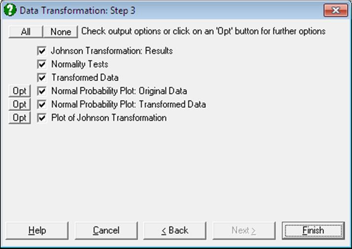
Transformed Data: The sorted original data, the transformed data and their group membership (if any) are displayed in a table. If you are using UNISTAT in Stand-Alone Mode, click on the UNISTAT icon on the Output Medium Toolbar to send all output to UNISTAT spreadsheet. In Excel Add-In Mode select the output matrix as data for further calculations.
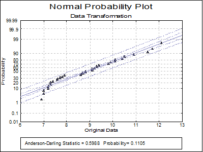
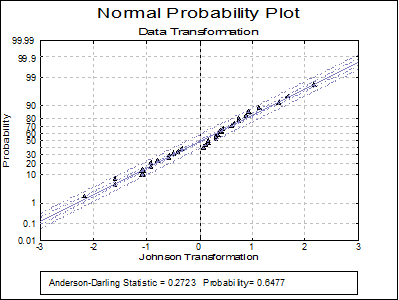
Normal Probability Plot of Original Data: A Normal Probability Plot of original data is displayed, together with its Anderson-Darling Test statistic and probability. You can compare this graph with the next one to visualise the improvement provided by the transformation.
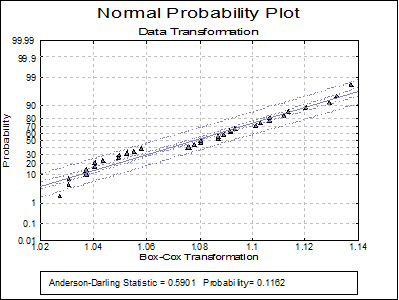
Normal Probability Plot of Transformed Data: A Normal Probability Plot of transformed data is displayed, together with its Anderson-Darling Test statistic and probability. You can compare this graph with the previous one to visualise the improvement provided by the transformation.
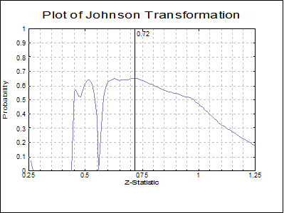
Plot of Johnson Transformation: Probabilities for Anderson-Darling Test on the transformed data are plotted against the z-values. The maximum probability is indicated on the graph. The curve generated may not always be continuous.
9.3.7.1.2. Johnson Transformation Example
Open REGRESS and select Statistics 2 → Quality Control → Data Transformation. From the Variable Selection Dialogue select cm (C2) as [Variable]. On Step 2 leave convergence parameters unchanged. On the Output Options Dialogue check all options to obtain the following output.
Data Transformation
Johnson Transformation: Results
Variables Selected: cm
|
Z-statistic for best fit = |
0.7200 |
|
Gamma = |
0.5500 |
|
Delta = |
0.6075 |
|
Xi = |
5.6319 |
|
Lambda = |
6.8365 |
Transformation selected: Johnson Bounded System (SB)
z = Gamma + Delta * LN((x – Xi) / (Xi + Lambda – x)), Xi < x < Xi + Lambda
z = 0.549976426928764 + 0.607452018062996 * LN((x – 6.83647857110731) / (5.63190833413029 + 6.83647857110731 – x))
Normality Tests
Smaller probabilities indicate non-normality.
|
|
A-D Stat |
Probability |
|
Original Data |
0.5988 |
0.1202 |
|
Transformed Data |
0.2723 |
0.6936 |
Transformed Data
|
|
Original Data |
Transformed Data |
|
1 |
6.9000 |
-2.1675 |
|
2 |
7.0000 |
-1.5821 |
|
3 |
7.0000 |
-1.5821 |
|
… |
… |
… |
|
31 |
11.5000 |
1.5048 |
|
32 |
11.7000 |
1.6709 |
|
33 |
12.1000 |
2.1654 |

9.3.7.2. Box-Cox Transformation
Box-Cox Transformation is a power transformation of the type:
![]()
![]()
The optimal value of lambda is determined by maximising the following log-likelihood function:
![]()
where ![]() is
the estimate of the variance of the transformed y variable.
is
the estimate of the variance of the transformed y variable.
The negative of the log likelihood function is minimised within a range defined by the user. The default range is -3 ≤ λ ≤ 3.
Box-Cox Transformation may not always provide a solution. The best way to find out whether a solution has been found is to ensure that the transformed data produces a higher Anderson-Darling Test probability than the original. Also, you will notice that in most cases Johnson Transformation provides a better transformation than Box-Cox Transformation.
9.3.7.2.1 Box-Cox Transformation Intermediary Inputs
This dialogue is similar to the Intermediate Inputs dialogue for Box-Cox Regression, except for the last item (see 7.2.9. Box-Cox Regression).
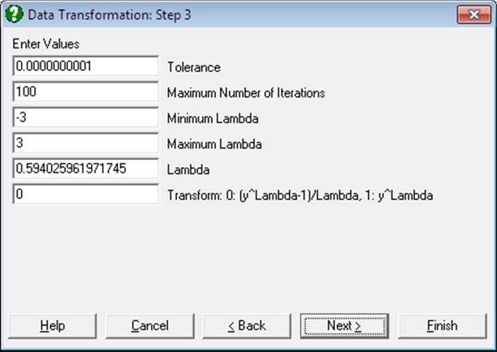
Tolerance: This value is used to control the sensitivity of minimisation procedure employed. Under normal circumstances, you do not need to edit this value. If a convergence cannot be achieved, then larger values of this parameter can be tried by removing one or more zeros.
Maximum Number of Iterations: When convergence cannot be achieved with the default value of 100 function evaluations, a higher value can be tried.
Minimum Lambda: Limits for the range where the optimum lambda will be search can be set. Change this value if the optimal lambda cannot be found within the specified range. If the lambda displayed is the same or very near to this minimum, change it to a smaller value. When the limit is changed, a re-calculation is forced and lambda is estimated again.
Maximum Lambda: Change this value if the optimal lambda cannot be found within the specified range. If the lambda displayed is the same or very near to this maximum, change it to a higher value. When the limit is changed, a re-calculation is forced and lambda is estimated again.
Lambda: You can override the estimated lambda and enter your own value here. You may wish to do this to use a round power value (like -1, -0.5, 0.5, 2). If the estimated lambda is changed, confidence intervals and chi-squared tests for lambda will not be available.
Transform: Once the optimal lambda is estimated using the standard Box-Cox Transformation, you will have a chance to generate the transformed variable using, (i) the same transformation:
![]()
![]()
or, (ii) the simple power transformation:
![]()
In some cases the second formula may be preferable to the first, since it will not generate nonpositive values. The choice made here will not affect normality of the transformed variable.
Remember that during the maximum likelihood estimation of lambda the original variable is always transformed using the first set of equations.
9.3.7.2.2 Box-Cox Transformation Output Options
This dialogue is similar to the maximum likelihood output dialogue for Box-Cox Regression (see 7.2.9.4. Box-Cox Regression Maximum Likelihood Output Options).
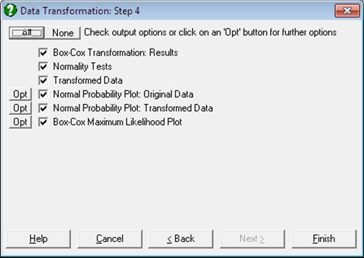
Box-Cox Transformation Results: This part of the output contains results for the maximum likelihood estimation.
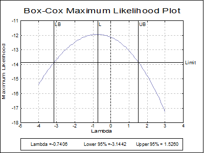
Lambda with Confidence Intervals: The confidence interval for optimum lambda is based on the likelihood ratio statistic and defined as:
![]()
Values corresponding to lower and upper bound of lambda are computed separately using an iterational procedure.
Likelihood Ratio Test: This test performed by evaluating the regression equation for lambda fixed at ![]() -1, 0 and 1.
-1, 0 and 1.
![]()
which is chi-square distributed with one degree of freedom.
Transformation Selected: The selected Box-Cox function is displayed. The two possibilities are:
![]()
and:
![]()
The equation is also printed on a separate line with estimated parameter values, in a format suitable for cell calculations in Excel. You can copy this equation, replace the variable x with a cell reference and run interpolations.
Normality Tests: The Anderson-Darling Test of normality is performed on the original and the transformed data thus allowing you to judge whether the transformation was useful. No or little increase in the tail probability indicates that the Box-Cox Transformation was not useful.
Transformed Data: The sorted original data, the transformed data and their group membership (if any) are displayed in a table. If you are using UNISTAT in Stand-Alone Mode, click on the UNISTAT icon on the Output Medium Toolbar to send all output to UNISTAT spreadsheet. In Excel Add-In Mode select the output matrix as data for further calculations.
Normal Probability Plot of Original Data: A Normal Probability Plot of original data is displayed, together with its Anderson-Darling Test statistic and probability. You can compare this graph with the next one to visualise the improvement provided by the transformation.
Normal Probability Plot of Transformed Data: A Normal Probability Plot of transformed data is displayed, together with its Anderson-Darling Test statistic and probability. You can compare this graph with the previous one to visualise the improvement provided by the transformation.
Box-Cox Maximum Likelihood Plot: Values of the log-likelihood function are plotted against lambda. The estimated lambda and its confidence intervals are also indicated.
9.3.7.2.3 Box-Cox Transformation Example
Open REGRESS and select Statistics 2 → Quality Control → Data Transformation. From the Variable Selection Dialogue select cm (C2) as [Variable]. On Step 2 leaving the convergence parameters unchanged produces an invalid lower bound for lambda. Change the minimum value for lambda from -3 to -4 and on the Output Options Dialogue check all options to obtain the following output.
Data Transformation
Box-Cox Transformation: Results
Variables Selected: cm
|
|
Value |
Lower 95% |
Upper 95% |
|
Lambda |
-0.7406 |
-3.1442 |
1.5260 |
Box-Cox Transformation:
y = (y ^ Lambda – 1) / Lambda
y = (POWER(y, -0.740557931816275) – 1) / -0.740557931816275
|
Lambda |
Chi-Square |
DoF |
Probability |
|
-1 |
0.0477 |
1 |
0.8272 |
|
0 |
0.3982 |
1 |
0.5280 |
|
1 |
2.2454 |
1 |
0.1340 |
|
Log of Likelihood = |
-11.9389 |
Normality Tests
Smaller probabilities indicate non-normality.
|
|
A-D Stat |
Probability |
|
Original Data |
0.5988 |
0.1202 |
|
Transformed Data |
0.5901 |
0.1264 |
Transformed Data
|
|
Original Data |
Transformed Data |
|
1 |
6.9000 |
1.0273 |
|
2 |
7.0000 |
1.0307 |
|
3 |
7.0000 |
1.0307 |
|
… |
… |
… |
|
31 |
11.5000 |
1.1291 |
|
32 |
11.7000 |
1.1319 |
|
33 |
12.1000 |
1.1372 |
