7.2.9. Box-Cox Regression
The ordinary least squares regression assumes normal distribution of residuals. When this is not the case, the Box-Cox Regression procedure may be useful (see Box, G. E. P. and Cox, D. R. 1964). It will transform the dependent variable using the Box-Cox Transformation function and employ maximum likelihood estimation to determine the optimal level of the power parameter lambda. In order to run a Box-Cox Regression, the dependent variable should not contain any non positive values.
Variable selection and Ordinary Least Squares Output dialogues for this procedure are identical to that of Linear Regression. There is a separate output dialogue for maximum likelihood estimation, which contains diagnostic and graphic options for the estimation parameters and normal probability plots of data before and after the transformation. It is possible to run a Box-Cox Regression without any independent variables. In this case the results will be similar to that of Data Transformation procedure with Box-Cox option (available under Statistics 2 → Quality Control menu).
7.2.9.1. Box-Cox Regression Model Description
Box-Cox Regression will transform the dependent variable as follows:
![]()
![]()
and determine the optimal value of lambda by maximising the following log-likelihood function:
![]()
where ![]() is
the estimate of the least squares variance using the transformed y variable.
is
the estimate of the least squares variance using the transformed y variable.
A golden section minimisation algorithm is employed to minimise the negative of the log likelihood function within the range of -3 ≤ λ ≤ 3. These limits can be changed by the user if necessary and the changes will be stored by the program.
7.2.9.2. Box-Cox Regression Variable Selection
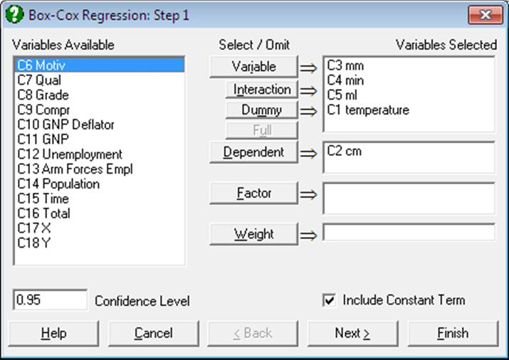
As in Linear Regression, Box-Cox Regression can be used to estimate models with or without a constant term, with or without weights and regressions can be run on a subset of cases as determined by the levels of an unlimited number of factor columns. An unlimited number of dependent variables can be selected in order to run the same model on different dependent variables. It is also possible to include interaction terms, dummy and lag/lead variables in the model, without having to create them as spreadsheet columns first (see 2.1.4. Creating Interaction, Dummy and Lag/Lead Variables).
It is compulsory to select at least one numeric data column as a dependent variable. When more than one dependent variable is selected, the analysis will be repeated as many times as the number of dependent variables, each time only changing the dependent variable and keeping the rest of selections unchanged.
You can transform a single variable without using any predictor (independent) variables. In this case the results will be similar to that of the Data Transformation procedure with Box-Cox option (available under Statistics 2 → Quality Control menu). A column containing numeric data can be selected as a weights column.
An intermediate inputs dialogue is displayed next.
7.2.9.3. Box-Cox Regression Intermediary Inputs
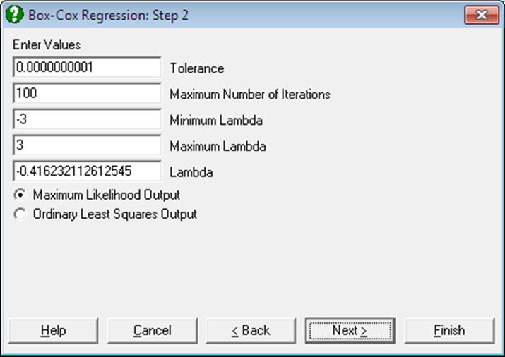
Tolerance: This value is used to control the sensitivity of minimisation procedure employed. Under normal circumstances, you do not need to edit this value. If convergence cannot be achieved, then larger values of this parameter can be tried by removing one or more zeros.
Maximum Number of Iterations: When convergence cannot be achieved with the default value of 100 function evaluations, a higher value can be tried.
Minimum Lambda: Limits for the range where the optimum lambda will be searched can be set. Change this value if the optimal lambda cannot be found within the specified range. If the lambda displayed is the same or very near to this minimum, change it to a smaller value. When the limit is changed, a re-calculation is forced and lambda is estimated again.
Maximum Lambda: Change this value if the optimal lambda cannot be found within the specified range. If the lambda displayed is the same or very near to this maximum, change it to a higher value. When the limit is changed, a re-calculation is forced and lambda is estimated again.
Lambda: You can override the estimated lambda and enter your own value here. You may wish to do this to use a round power value (like -1, -0.5, 0.5, 2). If the estimated lambda is changed, confidence intervals and chi-squared tests for lambda will not be available.
7.2.9.4. Box-Cox Regression Maximum Likelihood Output Options
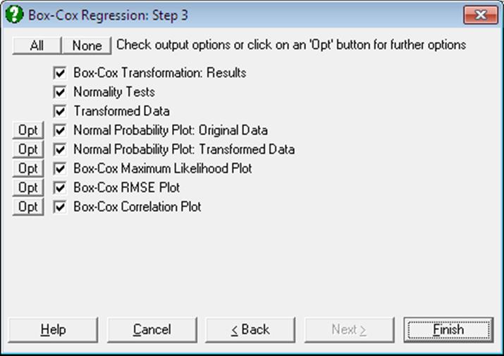
Box-Cox Transformation:
Results: The first output option displays results for the maximum likelihood estimation (see 9.3.7.2. Box-Cox Transformation).
Lambda with Confidence Limits: The confidence interval for optimum lambda is based on the likelihood ratio statistic and it is defined as:
![]()
Values corresponding to lower and upper bound of lambda are computed separately using an iterational procedure.
Transformation Formula: The equation applied in transforming the dependent variable is displayed. The same equation is also printed on a separate line with estimated parameter values, in a format suitable for cell calculations in Excel. You can simply copy this equation, replace the variable x with a cell reference and run interpolations.
Likelihood Ratio Test: In Box-Cox Regression, this test performed by evaluating the regression equation for lambda fixed at λ1 = -1, 0 and 1.
![]()
which is chi-square distributed with one degree of freedom.
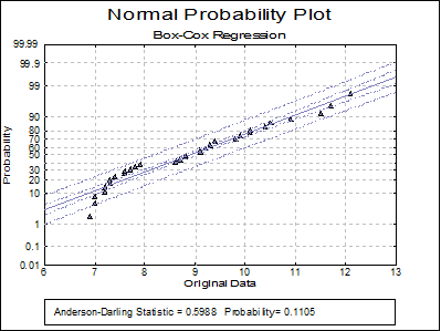
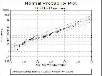
Normality Tests: Anderson-Darling Test of normality is performed on the original and transformed dependent variable thus allowing you to judge whether the transformation was useful. No or a small increase in the tail probability indicates that Box-Cox Transformation was not useful.
Transformed Data: The original and transformed dependent variable values and their group membership (if any) are sorted and displayed in a table. If you wish to display the unsorted values, you can use the Case (Diagnostic) Statistics output in Ordinary Least Squares Output option.
If you are using UNISTAT in Stand-Alone Mode, click on the UNISTAT icon on the Output Medium Toolbar to send all output to UNISTAT spreadsheet. In Excel Add-In Mode select the output matrix as data for further calculations.
Normal Probability Plot: Original Data: A Normal Probability Plot of the original data is displayed together with Anderson-Darling Test results in the legend. You can compare this graph with the next one to visualise the improvement provided by the transformation.
Normal Probability Plot: Transformed Data: A Normal Probability Plot of the transformed data is displayed together with Anderson-Darling Test results in the legend. You can compare this graph with the previous one to visualise the improvement provided by the transformation.
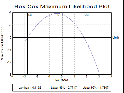
Box-Cox Maximum Likelihood Plot: Log likelihood values are plotted against the specified range of lambda. Lambda and its confidence limits are indicated by vertical lines. A horizontal line is drawn for the log likelihood value corresponding to confidence limits.
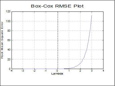
Box-Cox Root Mean Square Error Plot: Root mean square error (RMSE) of regression is plotted against lambda.
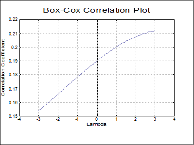
Box-Cox Correlation Plot: Values of the regression correlation coefficient are plotted against lambda.
7.2.9.5. Box-Cox Regression Ordinary Least Squares Output Options
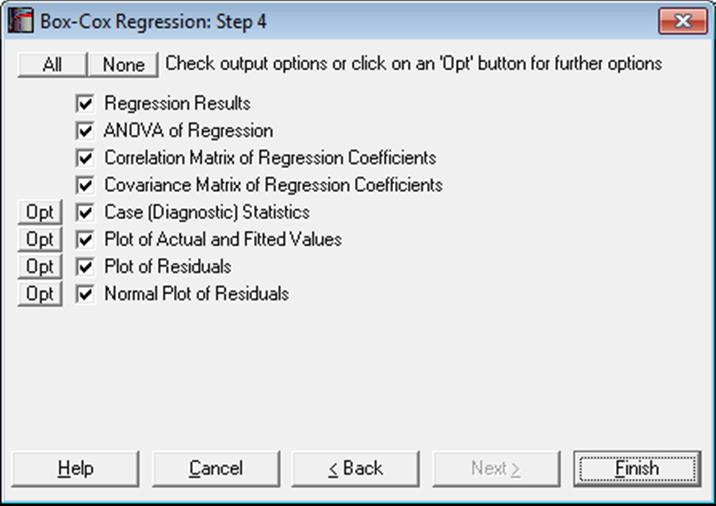
All output options are as in Linear Regression. The transformed dependent variable is used. The unsorted values for the transformed dependent variable can be accessed from the Case (Diagnostic) Statistics output option.
7.2.9.6. Box-Cox Regression Example
Open REGRESS and select Statistics 1 → Regression Analysis → Box-Cox Regression. From the Variable Selection Dialogue select temperature, mm, min and ml (C1, C3-C5) as [Variable]s and cm (C2) as [Dependent]. On Step 2 leave convergence parameters unchanged.
The Maximum Likelihood Output option generates the following output.
Box-Cox Regression
Box-Cox Transformation: Results
Variables Selected: cm
|
|
Value |
Lower 95% |
Upper 95% |
|
Lambda |
-0.4162 |
-2.7747 |
1.7807 |
Box-Cox Transformation:
y = (y ^ Lambda – 1) / Lambda
y = (POWER(y, -0.416232112612545) – 1) / -0.416232112612545
|
Lambda |
Chi-Square |
DoF |
Probability |
|
-1 |
0.2511 |
1 |
0.6163 |
|
0 |
0.1318 |
1 |
0.7165 |
|
1 |
1.5689 |
1 |
0.2104 |
|
Log of Likelihood = |
-8.0864 |
Normality Tests
Smaller probabilities indicate non-normality.
|
|
A-D Stat |
Probability |
|
Original Data |
0.5988 |
0.1202 |
|
Transformed Data |
0.5682 |
0.1434 |
Transformed Data
|
|
Original Data |
Transformed Data |
|
1 |
6.9000 |
1.3273 |
|
2 |
7.0000 |
1.3337 |
|
3 |
7.0000 |
1.3337 |
|
… |
… |
… |
|
31 |
11.5000 |
1.5332 |
|
32 |
11.7000 |
1.5394 |
|
33 |
12.1000 |
1.5514 |
Select the Ordinary Least Squares Output option and check only the Regression Results option to obtain the following ordinary least squares regression output.
Box-Cox Regression
Dependent Variable: cm
Valid Number of Cases: 33, 0 Omitted
Regression Results
|
|
Coefficient |
Standard Error |
t-Statistic |
Significance |
Lower 95% |
Upper 95% |
|
Constant |
1.6405 |
0.1886 |
8.6991 |
0.0000 |
1.2542 |
2.0268 |
|
temperature |
0.0054 |
0.0048 |
1.1318 |
0.2673 |
-0.0044 |
0.0153 |
|
mm |
-0.0436 |
0.0302 |
-1.4439 |
0.1599 |
-0.1055 |
0.0183 |
|
min |
0.0125 |
0.0114 |
1.0896 |
0.2852 |
-0.0110 |
0.0359 |
|
ml |
-0.0052 |
0.0285 |
-0.1813 |
0.8574 |
-0.0636 |
0.0532 |
|
Residual Sum of Squares = |
0.1150 |
|
Standard Error = |
0.0641 |
|
Mean of Y = |
1.4271 |
|
Standard Deviation of Y = |
0.0664 |
|
Correlation Coefficient = |
0.4305 |
|
R-squared = |
0.1854 |
|
Adjusted R-squared = |
0.0690 |
|
F(4,28) = |
1.5927 |
|
Significance of F = |
0.2038 |
|
Durbin-Watson Statistic = |
1.4016 |
|
Press Statistic = |
0.1800 |
