8.3. Multidimensional Scaling

This is, in a sense, the reverse of other multivariate methods. Instead of computing dissimilarities from raw data, Multidimensional Scaling (or MDS analysis) attempts to reconstruct the coordinates of points from a given dissimilarity matrix. A typical example is to reconstruct the locations of cities in a country from a given mileage chart. In general, Multidimensional Scaling methods will provide a satisfactory reconstruction of a map, except their orientation (rotation and reflection) and scaling.

The two general categories of Multidimensional Scaling are metric (or classical) and nonmetric (or ordinal) analyses, where the former attempts to reconstruct a map with correct distances, the latter concentrates on the relative positions of points, rather than their distances. The present implementation of Multidimensional Scaling analysis brings together these two methods in a single procedure. First a classical scaling is performed on the dissimilarity matrix, and then the derived configuration is input as initial values for the ordinal Multidimensional Scaling analysis.

A linear classical analysis should be performed before an ordinal one. The program will do this automatically, even if only the ordinal option is selected. It is, however, possible to obtain the classical and ordinal analysis results separately in two different Output Options Dialogues.

8.3.1. Classical Multidimensional Scaling

The Classical Multidimensional Scaling method was developed by Torgerson, W. S. (1958). It is a slight variation of principle components analysis and is also referred to as principle coordinates analysis.

First the proximity data is normalised and the normalised elements are squared:

  

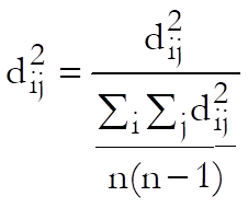
Then a scalar products matrix is formed:

  

where:

  

  

  

The classical scaling Output Options Dialogue displays a table and a graph.

Initial Coordinates: Eigenvectors of [bij], multiplied by the square root of the corresponding eigenvalues constitute the initial coordinates.

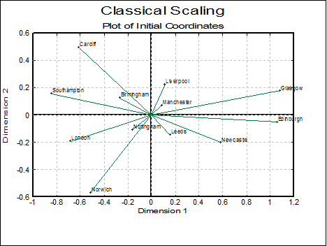
Plot of Initial Coordinates: A 2D plot of the initial coordinates is displayed.

8.3.2. Ordinal Multidimensional Scaling

In reality, a dissimilarity matrix is never an exact measure of the Euclidian distance between the points it represents. The general problem is better described in terms of the relative positions of points rather than their exact distances. For this purpose, the ordinal scaling methods rank distances in the original dissimilarity matrix and aim at obtaining coordinates of points whose ranked distances are the same as that of the original data.

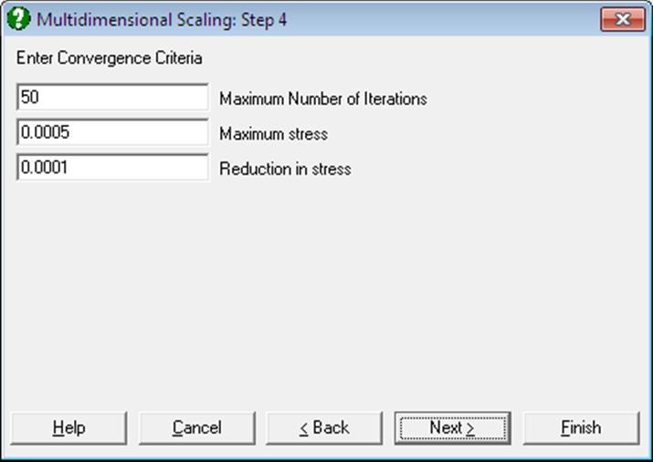
The ordinal multidimensional scaling procedure adopted here uses an iterational procedure known as monotonic least squares (see Kruskal, J. B. and Wish, M. 1978). This is a least squares (in this context also called stress) minimisation method, subject to the constraint that the solution should be in the same rank order as the original data. The convergence parameters for the monotonic least squares procedure can be controlled by the user.

Convergence History: The stress and reduction in stress values are displayed for each iteration. The reason for stopping iterations is also displayed.

Final Coordinates: The coordinates, when the iterations have been stopped, are displayed

Estimated Coefficients: n(n – 1)/2 coefficients for the least squares coefficients are displayed.

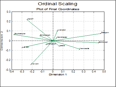
Plot of Final Coordinates: Final coordinates are plotted in 2D.

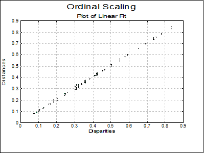
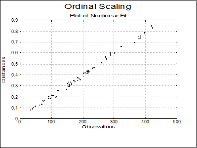
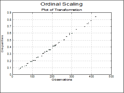
Plots of Linear Fit, Nonlinear Fit and Transformation: A scatter graph is plotted for each pair of the last three columns of the Estimated Coefficients table.

Example

The file UKCITIES contains a matrix which gives the distance (in miles) between twelve cities in the UK. This data is used to calculate a map showing the position of these cities relative to each other.

Open UKCITIES, select Statistics 2 → Multidimensional Scaling and select from Birmingham to Southampton (C1 to C12) as [Variable]s. Leave the default options on the second dialogue and then select the Classical Scaling option. Then select Plot of Initial Coordinates from the output dialogue and Dimension 2 as [X-Axis] and Dimension 1 as [Y-Axis].

The resulting map shows the calculated position of the twelve cities. This is actually a reflection (see 8.3. Multidimensional Scaling) down the y-axis of the true position of these cities, since Manchester is actually to the west of Leeds in the UK.

Continuing from the last example, click on the [Last Procedure Dialogue] button. Then click [Back] and select Ordinal Scaling. Accept the default values on the next two dialogues. The Estimated Coefficients table below is truncated to save space.

Ordinal Scaling

Convergence History

Terminated at iteration 1, since stress < 0.0005

Iteration	Stress	Reduction	%Reduction
1	0.0003	0.0002	48.18%

 

Final Coordinates

	Dimension 1	Dimension 2
Birmingham	-0.1263	0.0486
Cardiff	-0.2484	0.2156
Edinburgh	0.4462	-0.0230
Glasgow	0.4691	0.0754
Leeds	0.0641	-0.0582
Liverpool	0.0448	0.1018
London	-0.2972	-0.0738
Manchester	0.0372	0.0279
Newcastle	0.2607	-0.0888
Norwich	-0.2118	-0.2477
Nottingham	-0.0632	-0.0404
Southampton	-0.3750	0.0626

 

Estimated Coefficients

	Observed	Distances	Disparities	Differences
1	35.0000	0.0743	0.0743	0.0000
2	40.0000	0.0902	0.0902	0.0000
3	44.0000	0.1011	0.1011	0.0000
4	50.0000	0.1091	0.1091	0.0000
5	63.0000	0.1215	0.1215	0.0000
…	…	…	…	…