10.4. Four-Parameter Logistic Model
This procedure features two implementations of the 4PL method; (1) according to European Pharmacopoeia (1997-2017) and (2) as described in United States Pharmacopoeia (2010) chapters <1032>, <1033>, <1034>, <81> and <111>. It is possible to estimate the Full and Reduced USP models including outlier detection, plate effects, equivalence tests, outlier detection and multiple potency estimates with confidence limits. 96-well ELISA, as well as unbalanced designs are supported.
10.4.1. 4PL Variable Selection
The required data format is as described in section 10.0.1. Data Preparation (also see 10.0.2. Doses, Dilutions and Potency). Response data is stacked in a single column, a second column contains the dose level for each response and an optional categorical data column indicates which preparation a particular dose-response pair belongs to. By default, all models are based on Completely Randomised Design.
The optional [Plate] variable is usually used to isolate the plate effect (or replicates). If all dose/treatment groups (or cells) have an equal number of replicates (or if the design is balanced) then including the plate effect is equivalent to analysing the data with Randomised Block Design.
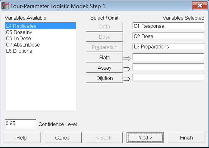
Designs can be unbalanced, i.e. the number of replicates for each dose-preparation combination may be different, dose levels for standard and test preparations may be different, there can be more than one test preparation, but the first five characters of the standard preparation label should be “stand” or “refer” in any language (capitalisation is not significant). Otherwise the first preparation encountered in the [Preparation] column will be considered as the standard.
Predictions (interpolations) can be obtained for response or dose values using the estimated model parameters. For details see section 10.0.7. Prediction, Interpolation, Extrapolation.
To run an analysis, it is sufficient to select one [Data] and one [Dose] variable. In this case, a single sigmoid curve will be fitted to data. If a [Preparation] variable (which should be a numeric or string factor or categorical data variable) is also selected, then you will have the option of fitting a Full Model (also known as Unconstrained Model) where a separate sigmoid curve is fitted for each preparation or a Reduced Model (also known as Constrained Model) where parallel sigmoid curves are fitted for selected preparations.
The next dialogue asks for the following convergence and model options.
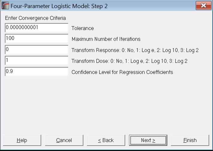
Tolerance: This value is used to control the sensitivity of the maximum likelihood procedure employed. Under normal circumstances, you do not need to edit this value. If convergence cannot be achieved, then larger values of this parameter can be tried by removing one or more zeros.
Maximum Number of Iterations: When convergence cannot be achieved with the default value of 100 function evaluations, a higher value can be tried.
Transform Response: It is possible to transform the response variable by one of e (natural), 10 or 2-based logarithms or leave it untransformed (default).
Transform Dose: It is possible to transform the dose variable by one of natural (default), 10 or 2-based logarithms or leave it untransformed.
Confidence Level for Regression Coefficients: While the general level of confidence (default 95%) is set on the Variable Selection Dialogue, confidence level for Regression Coefficients and Equivalence Tests can be set here separately. The default is 90%.
In the next dialogue, the model to be estimated is selected.
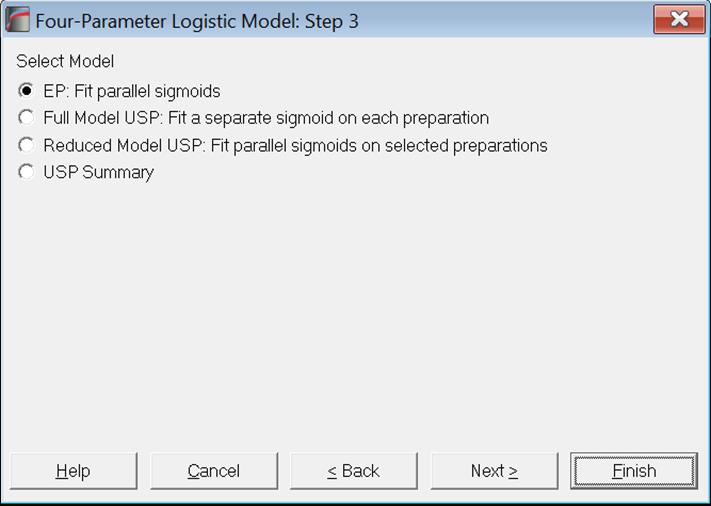
EP: Parallel sigmoid curves are fitted for all preparations. Validity tests based on weighted sums of squares and fiducial confidence limits of estimated potency are reported according to European Pharmacopoeia (1997-2017). See sections 10.3.2.5. Potency and 10.4.2.1. EP (European Pharmacopoeia).
Full Model USP: This is also known as the unrestricted, unconstrained or nonparallel model. A separate sigmoid curve is fitted for each preparation. See section 10.4.2.2. Full Model USP.
Reduced Model USP: Also known as the restricted, constrained or parallel model. Parallel sigmoid curves are fitted for all selected preparations.
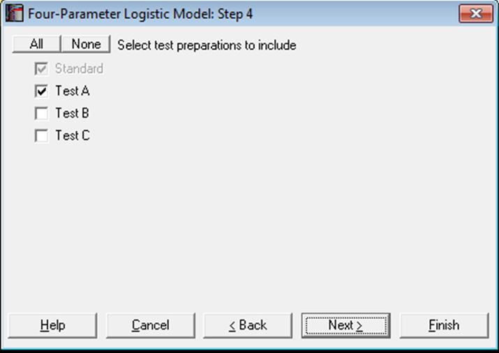
If Reduced Model USP is selected, then a further dialogue will allow you to select the test preparations to include in the model. Goodness of Fit and Equivalence Tests options can be used to determine which preparations should be included.
USP Summary: UNISTAT implements Full and Reduced models as two separate procedures since each has a large number of diagnostic and equivalence tests. As of this version, we add a USP Summary option which combines the basic output from the two models in a single report. See section 10.4.2.4. USP Summary.
10.4.2. 4PL Output Options
The 4-parameter logistic function is given as:
![]()
where:
A is upper asymptote,
D is lower asymptote,
B is Hill slope,
C is ED50 and
x is the random variable dose.
In the output, these parameters will be labelled by their above string literals. If this is not the terminology you are used to, you can change these by entering the following line:
4plLabels=i
C:\ProgramData\Unistat\Unistat10\Unistat10.ini
The parameter labels used will be:
for i = 0: Upper asymptote, Lower asymptote, Hill slope, ED50 (default),
for i = 1: A, D, B, EC50,
for i = 2: Top, Bottom, Hill, EC50.
10.4.2.1. EP (European Pharmacopoeia)
Parallel sigmoid curves are fitted for all preparations. European Pharmacopoeia approach is similar to Reduced Model USP in many respects, with two significant differences;
- EP reports fiducial limits of potency whereas USP reports confidence limits based on the standard error and t-interval and
- EP tests validity of assay using weighted sums of squares and chi-square tests whereas USP recommends either equivalence tests or F-tests based on the difference in residual sums of squares between the Full and Reduced models.
Four-Parameter Logistic Model according to European Pharmacopoeia has the following output options.
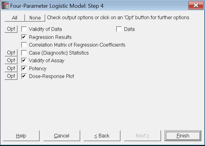
Validity of Data: A wide range of statistics on treatment groups are reported, including detection of outliers. This menu item is identical to the same one available under Parallel Line Method. For details see section 10.1.2.1. Validity of Data.
Regression Coefficients: The t-statistic is defined as:
![]()
and has a t-distribution with:
df = N – (3 + k)
degrees of freedom and N is the total number of observations used in the analysis, including all preparations.
Confidence intervals for regression coefficients are computed as:
![]()
where each coefficient’s standard error σj is the square root of the diagonal element of the covariance matrix:
![]()
where X is the Jacobian matrix. See Seber, G A. F. and Wild, C. J 2003.
Correlation Matrix of Regression Coefficients: This is a symmetric matrix with unity diagonal elements. It gives the correlation between regression coefficients and is obtained by dividing each element of (X’X)-1 matrix by the square root of the diagonal elements corresponding to its row and column.
Case (Diagnostic) Statistics:
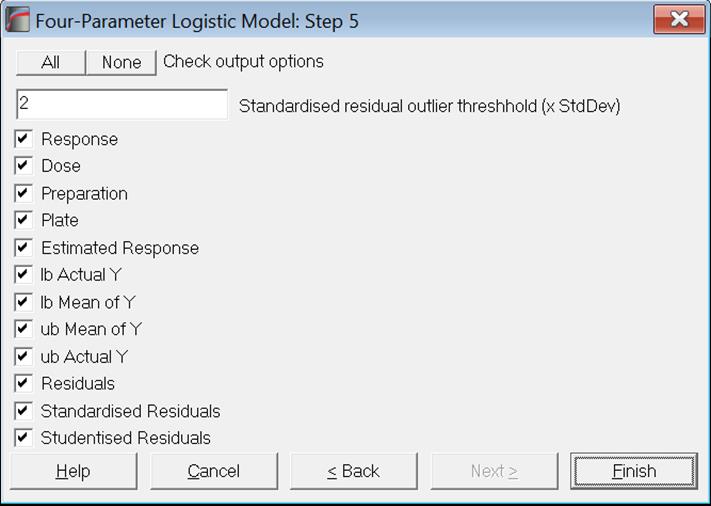
Prediction (interpolation) and outlier detection: See sections 10.0.6.2. Model-Based Outlier Detection and 10.0.7. Prediction, Interpolation, Extrapolation.
Confidence and Prediction Intervals: Approximate standard errors are calculated using the delta method (Van Der Vaart, 1998). Defining the column vector of partial derivatives with respect to each parameter as:
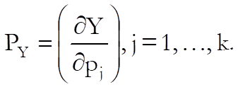
for each given level of dose calculate:
![]()
The standard error for actual Y (confidence) for that dose level is:
![]()
and the standard error for mean of Y (prediction) is:
![]()
The 95% intervals are then calculated as:
![]()
Validity of Assay: The following tests for model fit (or lack of fit) are provided.
Weighted ANOVA: Sum of squares are weighted as defined in Finney, D. J. (1978) p. 372.
Non-linearity test:
![]()
Non-parallelism test:

with (m – 1) degrees of freedom.
Total sum of squares:
![]()
with N – 1 degrees of freedom.
Residual sum of squares:
![]()
where y-bar is the mean response for each preparation and y-hat is the overall mean of all responses.
Chi-square statistics are obtained by dividing SSQs with Rssqw / DoF(Rssqw).
Weighted R-squared:
![]()
ANOVA of Regression: For each preparation the total sum of squares is:
![]()
with N – 1 degrees of freedom and the residual sum of squares is:
![]()
The unweighted R-squared value is calculated as
![]()
Example
Weighted ANOVA
|
|
Sum of Squares |
Chi-Square |
DoF |
Probability |
Pass/Fail |
|
Preparations |
0.001 |
0.530 |
1 |
0.4667 |
Pass |
|
Regression |
9.432 |
6600.317 |
1 |
0.0000 |
Pass |
|
Non-parallelism |
0.000 |
0.046 |
1 |
0.8306 |
Pass |
|
Non-linearity |
0.013 |
8.894 |
16 |
0.9177 |
Pass |
|
Standard S Non-linearity |
0.008 |
5.355 |
8 |
0.7191 |
Pass |
|
Preparation T Non-linearity |
0.005 |
3.539 |
8 |
0.8961 |
Pass |
|
Treatments |
9.445 |
6609.786 |
19 |
0.0000 |
Pass |
|
Residual |
0.029 |
|
20 |
|
|
|
Total |
9.474 |
|
39 |
|
|
|
R-squared |
0.996 |
|
|
|
Pass |
ANOVA of Regression
|
Due To |
Sum of Squares |
DoF |
Mean Square |
F-Stat |
Prob |
Pass/Fail |
|
Regression |
42.193 |
4 |
10.548 |
8927.664 |
0.0000 |
Pass |
|
Error |
0.041 |
35 |
0.001 |
|
|
|
|
Total |
42.235 |
39 |
1.083 |
|
|
|
|
R-squared |
0.999 |
|
|
|
|
Pass |
Potency:
The relative potency for test preparation i is found as:
![]()
where ![]() and
and ![]() are the intercepts for test i and
standard preparations and
are the intercepts for test i and
standard preparations and ![]() is
the common slope.
is
the common slope.
To calculate the confidence limits of Mi first define:
![]()
First define:
![]()
![]()
The fiducial confidence interval for potency ratio of each test preparation is defined as:
![]()
where:
![]()
Mi is the relative potency and MiL and MiU are the confidence limits for the relative potency. The estimated potency and its confidence interval are obtained by multiplying these relative values by the assumed potency supplied by the user for each test preparation separately.
The approximate variance of Mi is:
![]()
Weights are computed after the estimated potency and its confidence interval are found:
![]()
and % Precision is:
![]()
If the data column [Dose] contains the actual dose levels administered in original dose units, we will obtain the estimated potency and its confidence limits in the same units. If, however, the [Dose] column contains unitless relative dose levels, then we may need to perform further calculations to obtain the estimated potency in original units. To do that you can enter assigned potency of the standard, assumed potency of each test preparation and pre-dilutions for all preparations including the standard in a data column and select it as [Dilution] variable. UNISTAT will then calculate the estimated potency as described in section 10.0.2. Doses, Dilutions and Potency. Also see section 10.0.3. Potency Calculation Example.
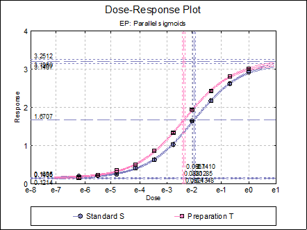
Dose-Response Plot: A dose-response curve will be drawn for all preparations. Selecting Edit → Dose-Response Plot… (or double-clicking on the graph area) will pop a dialogue where what is displayed on the plot can be controlled.
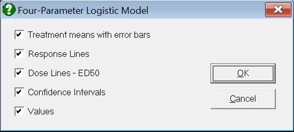
For each curve it is possible to draw lines for ED50, asymptotes, and their confidence limits with or without values. By default, confidence limits for actual Y values (i.e. the confidence interval) are drawn for each curve. If you wish to display the prediction interval instead, enter the following line:
4plPredictionInterval=1
C:\ProgramData\Unistat\Unistat10\Unistat10.ini
10.4.2.2. Full Model USP
A separate sigmoid curve is fitted for each preparation. Therefore, this model has 4k parameters, where k is the number of preparations including the standard (or reference). This is also known as the unrestricted, unconstrained or nonparallel model.
Validity of Data: A wide range of statistics on treatment groups are reported, including detection of outliers. This menu item is identical to the same one available under Parallel Line Method. For details see section 10.1.2.1. Validity of Data.
Regression Coefficients: The t-statistic is defined as:
![]()
and has a t-distribution with:
df = N – (4 * k)
degrees of freedom and N is the total number of observations used in the analysis, including all preparations. When a plate factor is selected, a Satterthwaite approximation of degrees of freedom is used as recommended by USP <1034>.
Confidence intervals for regression coefficients are computed as:
![]()
where each coefficient’s standard error σj is the square root of the diagonal element of the covariance matrix:
![]()
where X is the Jacobian matrix. See Seber, G A. F. and Wild, C. J 2003.
Correlation Matrix of Regression Coefficients: This is a symmetric matrix with unity diagonal elements. It gives the correlation between regression coefficients and is obtained by dividing each element of (X’X)-1 matrix by the square root of the diagonal elements corresponding to its row and column.
Case (Diagnostic) Statistics:
Prediction (interpolation) and outlier detection: See sections 10.0.6.2. Model-Based Outlier Detection and 10.0.7. Prediction, Interpolation, Extrapolation.
Confidence and Prediction Intervals: Approximate standard errors are calculated using the delta method (Van Der Vaart, 1998). Defining the column vector of partial derivatives with respect to each parameter as:
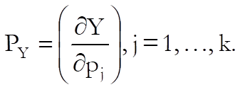
for each given level of dose calculate:
![]()
The standard error for actual Y (confidence) for that dose level is:
![]()
and the standard error for mean of Y (prediction) is:
![]()
The 95% intervals are then calculated as:
![]()
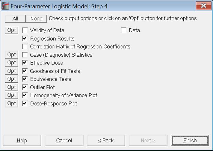
Effective Dose: ED50 is readily estimated as a model parameter together with its standard error and 90% confidence limits. If you need to obtain other effective dose values for the currently estimated model (i.e. the so-called EDanything), you can enter or edit the ED values from this dialogue, which pops up when you click the [Opt] button situated to the left of the Effective Dose option.
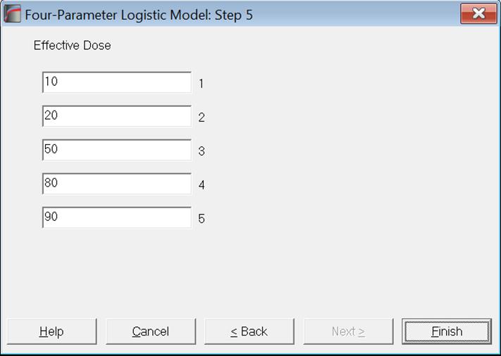
For a given percentage point P% the effective dose is calculated as:
![]()
Approximate standard errors are calculated using the delta method (Van Der Vaart, 1998). Defining the column vector of partial derivatives with respect to each parameter as:
![]()
for each given level of effective dose calculate:
![]()
The standard error for that effective dose is:
![]()
and the 90% intervals are then calculated as:
![]()
Goodness of Fit tests: The following measures of model fit (or lack of fit) are provided. The first option Validity of Assay is not available for the Full Model.
ANOVA of Regression: For each preparation the total sum of squares is:
![]()
with N – 1 degrees of freedom and the residual sum of squares is:
![]()
with 3 degrees of freedom (i.e. four parameters less one). Here y-bar is the mean response for each preparation and y-hat is the overall mean of all responses.
The R-squared value is calculated as:
![]()
Measures of Variability: Let σ2 be the total variance of residuals. Then:
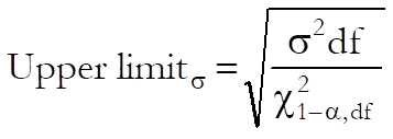
where the degrees of freedom is the same as in the Regression Coefficients output.
Upper limit of geometric standard deviation (GSD) is:
![]()
upper limit of the percent geometric coefficient of variation (%GCV) is:
![]()
and upper limit of the percent coefficient of variation (%CV) is calculated as:
![]()
If a [Plate] column is selected, the total variance is broken into within and between plate components and the one-sided upper 95% limits are also computed for within plate standard deviation.
Equivalence Tests: These tests are used to decide which test preparations are to be included in the Reduced Model as recommended by USP <1034>.
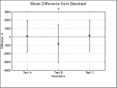
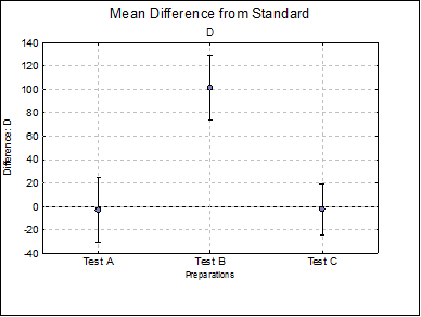
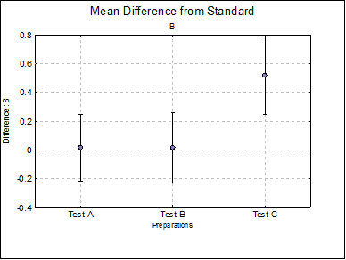
Mean Difference from Standard: For each model parameter other than ED50 (i.e. A, D and B), the difference between the standard and each test preparation and their confidence limits are tabulated. For instance, for the upper asymptote A:
![]()
![]()
The 90% intervals are then calculated as:
![]()
The criteria against which an accept or reject decision is to be made (i.e. the so-called goalposts) are not included here. These criteria must be based on the specific properties of the bioassay.
Difference Plots: Three plots for parameters A, D and B are displayed with error bars. Each plot will have k – 1 points, one for each test preparation.
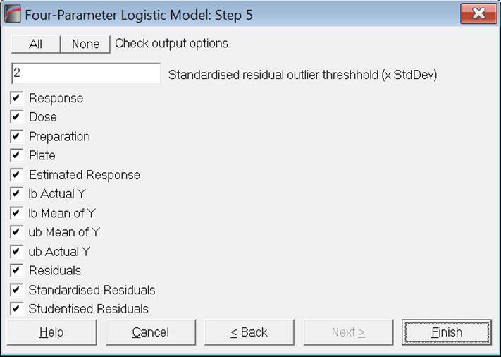
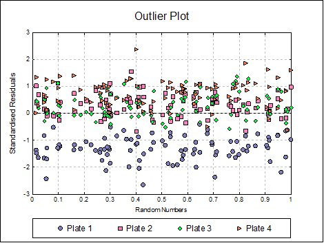
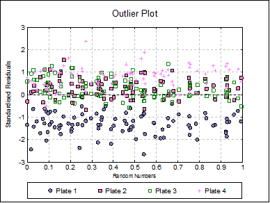
Outlier Plot: Standardised residuals are plotted against a randomized X-axis. If a [Plate] factor has been selected, the residuals are marked by their plate membership, otherwise by preparation.
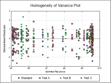
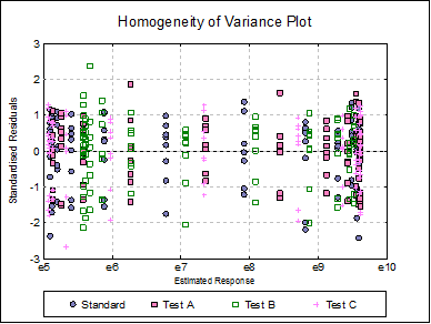
Homogeneity of Variance Plot: Studentised residuals are plotted against estimated (fitted) response values. Residuals are marked by their preparation membership. If the horizontal spread of points indicates a bias, the response variable may need to be transformed to improve the homogeneity of variance.
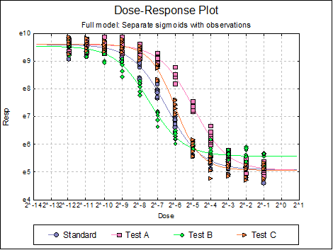
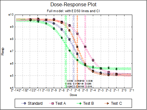
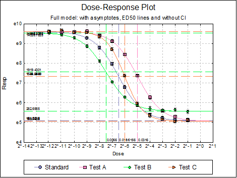
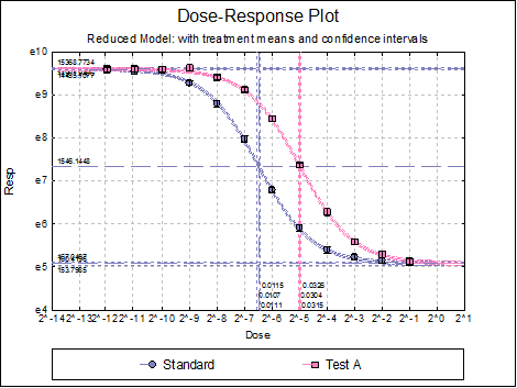
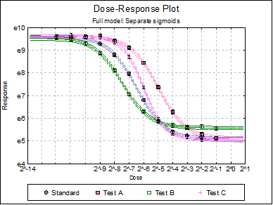
Dose-Response Plot: A dose-response curve will be drawn for each preparation. Selecting Edit → Dose-Response Plot… (or double-clicking on the graph area) will pop a dialogue where what is displayed on the plot can be controlled.
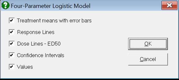
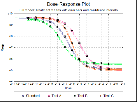
For each curve it is possible to draw lines for ED50, asymptotes, and their confidence limits with or without values By default, confidence limits for actual Y values (i.e. the confidence interval) are drawn for each curve. If you wish to display the prediction interval instead, enter the following line:
4plPredictionInterval=1
C:\ProgramData\Unistat\Unistat10\Unistat10.ini
Here are a few examples of what can be achieved:
10.4.2.3. Reduced Model USP
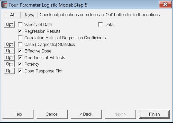
This is also known as the restricted, constrained or parallel model. USP <1034> recommends that the best subset of preparations to be included in Reduced Model should be selected using Equivalence Tests as described in Full Model output above.
This model assumes that all preparations have the same A, D and B coefficients and only differ in parameter C (i.e. ED50). Therefore, the Reduced Model has 3 + k’ parameters to estimate; A, D, B, Cj j = 1, …, k’, where k’ is the number of preparations selected, including the standard.
Validity of Data: A wide range of statistics on treatment groups are reported, including detection of outliers. This menu item is identical to the same one available under Parallel Line Method. For details see section 10.1.2.1. Validity of Data.
Regression Coefficients: The t-statistic is defined as in Full Model, except for the degrees of freedom, which is for Reduced Model:
df = N’ – (3 + k)
where N’ is the total number of observations used in Reduced Model.
Correlation Matrix of Regression Coefficients: Correlations between all 3 + k’ parameters are displayed.
Case (Diagnostic) Statistics: These are as described in Full Model.
Effective Dose: You can obtain effective dose values other than 50% and their confidence limits as described in Full Model.
Goodness of Fit tests: The first option Validity of Assay is based on the description given by Gottschalk, P. G. and Dunn, J. R. (2005). The remaining two options, ANOVA of Regression and Measures of Variability are as in Full Model.
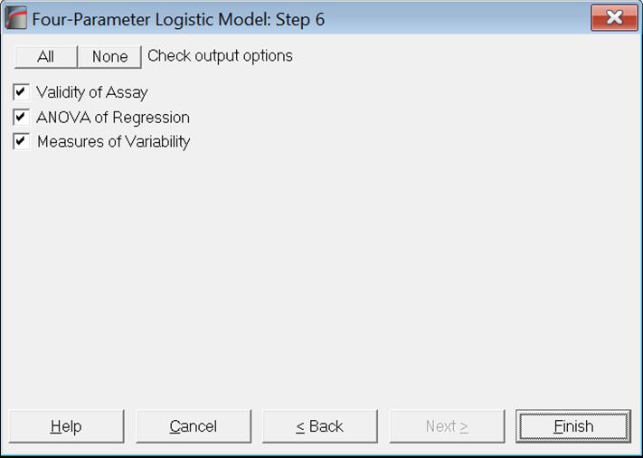
Validity of Assay: This option is only available for USP Reduced Model and parallelism and linearity tests are available only when it is run immediately after a Full Model. This is because the parallelism and linearity tests here depend on the difference in residual sum of squares for Full and Reduced models. The USP Summary option performs the two models consecutively and therefore parallelism and linearity tests are always available under this output option. See section 10.4.2.4. USP Summary.
The sum of squares for the non-parallelism test is the difference between residual SSQ of the Reduced model minus sum of all residual SSQs of the Full model:
![]()
with:
df = (4 * k’) – (3 + k’)
degrees of freedom, where k’ is the number of preparations selected in Reduced Model.
The non-linearity test is defined as the difference between weighted non-linearity SSQ and sum of all residual SSQs of the Full model. For details see Gottschalk, P. G. and Dunn, J. R. (2005).
Example
Validity of Assay
|
Due To |
Sum of Squares |
DoF |
Mean Square |
F-Stat |
Prob |
Pass/Fail |
|
Preparations |
0.231 |
1 |
0.231 |
161.363 |
0.0000 |
Pass |
|
Regression |
41.963 |
3 |
13.988 |
9788.536 |
0.0000 |
Pass |
|
Non-parallelism |
0.002 |
3 |
0.001 |
0.489 |
0.6937 |
Pass |
|
Non-linearity |
0.011 |
12 |
0.001 |
0.619 |
0.8022 |
Pass |
|
Treatments |
42.206 |
19 |
2.221 |
1554.519 |
0.0000 |
Pass |
|
Residual |
0.029 |
20 |
0.001 |
|
|
|
|
Total |
42.235 |
39 |
1.083 |
|
|
|
|
R-squared |
0.999 |
|
|
|
|
Pass |
Potency: In transformed (logged) scale, the relative potency for test preparation j is found as:
![]()
and its confidence limits as:
![]()
where the variance of relative potency for test preparation j is:
![]()
The relative potency and its confidence limits are then transferred (anti-logged) back to the original scale.
Weights (which are needed when various potencies are to be combined) are computed as:
![]()
and % Precision is:
![]()
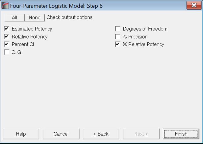
If the data column [Dose] contains the actual dose levels administered in original dose units, we will obtain the estimated potency and its confidence limits in the same units. If, however, the [Dose] column contains unitless relative dose levels, then we may need to perform further calculations to obtain the estimated potency in original units. To do that you can enter assigned potency of the standard, assumed potency of each test preparation and pre-dilutions for all preparations including the standard in a data column and select it as [Dilution] variable. UNISTAT will then calculate the estimated potency as described in section 10.0.2. Doses, Dilutions and Potency. Also see section 10.0.3. Potency Calculation Example.
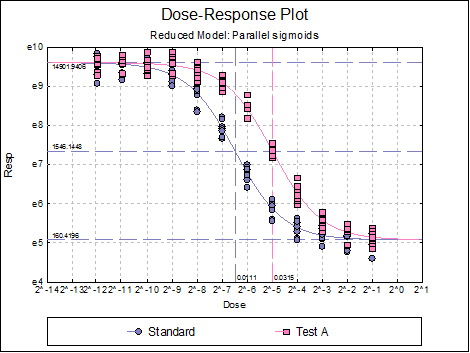
Dose-Response Plot: This has the same options as the dose-response plot described for the Full Model in the previous section.
10.4.2.4. USP Summary
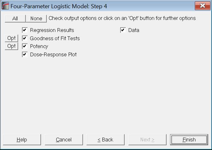
As we have seen in previous sections, USP recommends equivalence tests in order to assess validity of assays which require running Full and Reduced models consecutively. Classic parallelism and linearity tests are also based on the difference in residual sums of squares between the Full and Reduced models. Under this menu item we provide a procedure combining the two models in a single run, generating a combined report. Details are as in sections 10.4.2.2. Full Model USP and 10.4.2.3. Reduced Model USP.
Note that this dialogue does not have an [Opt] button for Dose-Response Plot option. This is because the output has two plots for Full and Reduced models. If you wish to edit these grapsh, you will need to run Full and Reduced models separately.
10.4.3. 4PL Examples
Example 1
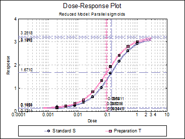
Data is given in Table 5.4.1.-I. on p. 4373 of European Pharmacopoeia (9th Edition).
Open BIOPHARMA9 and select Bioassay → Four-Parameter Logistic Model. From the Variable Selection Dialogue select columns C44, C45, L46 and L47 respectively as [Data], [Dose], [Preparation] and [Dilution]. Click [Next] and leave all entries on the Convergence Criteria dialogue unchanged. On the next two dialogues select EP: Fit parallel sigmoids and check Preparation T. On Output Options Dialogue check only the Regression Results and Potency options.
Click [Finish] to obtain the following output. Note that the potency reported here is relative potency.
Four-Parameter Logistic Model
Valid Number of Cases: 40, 0 Omitted
Model selected: EP
Regression Results
|
|
Coefficient |
Standard Error |
t-Statistic |
2-Tail Probability |
Lower 90% |
Upper 90% |
|
Upper asymptote |
3.1960 |
0.0327 |
97.7429 |
0.0000 |
3.1407 |
3.2512 |
|
Lower asymptote |
0.1455 |
0.0143 |
10.2042 |
0.0000 |
0.1214 |
0.1695 |
|
Hill slope |
1.1244 |
0.0294 |
38.2340 |
0.0000 |
1.0747 |
1.1741 |
|
Standard S ED50 |
0.1348 |
0.0037 |
36.4278 |
0.0000 |
0.1285 |
0.1410 |
|
Preparation T ED50 |
0.0924 |
0.0026 |
35.7697 |
0.0000 |
0.0880 |
0.0967 |
|
Total Residual Variance = |
0.0012 |
|
Degrees of Freedom = |
35 |
Weighted ANOVA
|
|
Sum of Squares |
Chi-Square |
DoF |
Probability |
|
Preparations |
0.001 |
0.530 |
1 |
0.4667 |
|
Regression |
9.432 |
6600.317 |
1 |
0.0000 |
|
Non-parallelism |
0.000 |
0.046 |
1 |
0.8306 |
|
Non-linearity |
0.013 |
8.894 |
16 |
0.9177 |
|
Standard S Non-linearity |
0.008 |
5.355 |
8 |
0.7191 |
|
Preparation T Non-linearity |
0.005 |
3.539 |
8 |
0.8961 |
|
Treatments |
9.445 |
6609.786 |
19 |
0.0000 |
|
Residual |
0.029 |
|
20 |
|
|
Total |
9.474 |
|
39 |
|
|
R-squared |
0.996 |
|
|
|
ANOVA of Regression
|
Due To |
Sum of Squares |
DoF |
Mean Square |
F-Stat |
Prob |
|
Regression |
42.193 |
4 |
10.548 |
8927.664 |
0.0000 |
|
Error |
0.041 |
35 |
0.001 |
|
|
|
Total |
42.235 |
39 |
1.083 |
|
|
|
R-squared |
0.999 |
|
|
|
|
Potency
Assigned potency of Standard S: 0.4 IU/ml
|
|
Estimated Potency |
Lower 95% |
Upper 95% |
|
Preparation T |
0.5835 |
0.5568 |
0.6116 |
|
|
Relative Potency |
Lower 95% |
Upper 95% |
|
Preparation T |
145.89% |
139.20% |
152.90% |
|
|
Percent CI |
Lower 95% |
Upper 95% |
|
Preparation T |
100.00% |
95.42% |
104.81% |
Example 2
Open the file 4PL and select Bioassay → Four-Parameter Logistic Model. From the Variable Selection Dialogue select columns C1 to C4 respectively as [Data], [Dose], [Preparation] and [Plate]. Click [Next], enter 1 for Transform Response, 3 for Transform Dose and leave other entries unchanged. On the next dialogue select Full Model: Fit a separate sigmoid on each preparation. Leave Output Options Dialogue unchanged and then click [Finish].
Four-Parameter Logistic Model
Valid Number of Cases: 384, 0 Omitted
Model selected: Full Model USP
Full Model USP
Regression Results
|
|
Coefficient |
Standard Error |
t-Statistic |
2-Tail Prob |
Lower 90% |
Upper 90% |
|
Standard A |
14851.5573 |
721.5338 |
20.5833 |
0.0000 |
13377.0205 |
16326.0941 |
|
D |
161.5165 |
7.8716 |
20.5189 |
0.0000 |
145.4300 |
177.6030 |
|
B |
-1.4833 |
0.0782 |
-18.9697 |
0.0000 |
-1.6431 |
-1.3235 |
|
EC50 |
0.0111 |
0.0004 |
25.8819 |
0.0000 |
0.0102 |
0.0120 |
|
Test A A |
14945.5751 |
577.3904 |
25.8847 |
0.0000 |
13765.6117 |
16125.5385 |
|
D |
158.2746 |
10.9899 |
14.4018 |
0.0000 |
135.8155 |
180.7337 |
|
B |
-1.5004 |
0.0828 |
-18.1187 |
0.0000 |
-1.6696 |
-1.3312 |
|
EC50 |
0.0316 |
0.0013 |
24.2711 |
0.0000 |
0.0289 |
0.0343 |
|
Test B A |
14027.4183 |
838.3262 |
16.7326 |
0.0000 |
12314.2027 |
15740.6339 |
|
D |
262.6613 |
10.8566 |
24.1937 |
0.0000 |
240.4746 |
284.8480 |
|
B |
-1.4996 |
0.0917 |
-16.3570 |
0.0000 |
-1.6869 |
-1.3122 |
|
EC50 |
0.0056 |
0.0003 |
22.2848 |
0.0000 |
0.0051 |
0.0061 |
|
Test C A |
14995.9650 |
578.6668 |
25.9147 |
0.0000 |
13813.3931 |
16178.5369 |
|
D |
159.0249 |
7.1096 |
22.3675 |
0.0000 |
144.4955 |
173.5542 |
|
B |
-2.0018 |
0.1060 |
-18.8896 |
0.0000 |
-2.2184 |
-1.7852 |
|
EC50 |
0.0156 |
0.0005 |
33.5103 |
0.0000 |
0.0147 |
0.0166 |
|
Total Residual Variance = |
0.0451 |
|
Degrees of Freedom = |
368 |
|
Satterthwaite DoF = |
4.7019 |
Correlation Matrix of Regression Coefficients
|
|
A |
D |
B |
EC50 |
|
Standard A |
1.0000 |
-0.2339 |
-0.5689 |
-0.4288 |
|
D |
-0.2339 |
1.0000 |
0.5698 |
-0.4309 |
|
B |
-0.5689 |
0.5698 |
1.0000 |
-0.0015 |
|
EC50 |
-0.4288 |
-0.4309 |
-0.0015 |
1.0000 |
|
Test A A |
1.0000 |
-0.2417 |
-0.4974 |
-0.2356 |
|
D |
-0.2417 |
1.0000 |
0.6673 |
-0.6290 |
|
B |
-0.4974 |
0.6673 |
1.0000 |
-0.2818 |
|
EC50 |
-0.2356 |
-0.6290 |
-0.2818 |
1.0000 |
|
Test B A |
1.0000 |
-0.2347 |
-0.6275 |
-0.5546 |
|
D |
-0.2347 |
1.0000 |
0.5172 |
-0.3068 |
|
B |
-0.6275 |
0.5172 |
1.0000 |
0.1771 |
|
EC50 |
-0.5546 |
-0.3068 |
0.1771 |
1.0000 |
|
Test C A |
1.0000 |
-0.1421 |
-0.4344 |
-0.3558 |
|
D |
-0.1421 |
1.0000 |
0.4831 |
-0.4325 |
|
B |
-0.4344 |
0.4831 |
1.0000 |
-0.0532 |
|
EC50 |
-0.3558 |
-0.4325 |
-0.0532 |
1.0000 |
Case (Diagnostic) Statistics
|
|
LogE (Response) |
Dose |
Preparation |
Plate |
Estimated Response |
95% lb Actual Y |
95% lb Mean of Y |
|
** 1 |
4.5962 |
0.5000 |
Standard |
Plate 1 |
5.1005 |
0.5007 |
4.1345 |
|
2 |
4.9461 |
0.5000 |
Standard |
Plate 1 |
5.1005 |
0.5007 |
4.1345 |
|
3 |
5.2660 |
0.5000 |
Standard |
Plate 2 |
5.1005 |
0.5007 |
4.1345 |
|
4 |
5.1606 |
0.5000 |
Standard |
Plate 2 |
5.1005 |
0.5007 |
4.1345 |
|
5 |
5.2318 |
0.5000 |
Standard |
Plate 3 |
5.1005 |
0.5007 |
4.1345 |
|
6 |
5.0652 |
0.5000 |
Standard |
Plate 3 |
5.1005 |
0.5007 |
4.1345 |
|
7 |
5.2122 |
0.5000 |
Standard |
Plate 4 |
5.1005 |
0.5007 |
4.1345 |
|
8 |
5.3453 |
0.5000 |
Standard |
Plate 4 |
5.1005 |
0.5007 |
4.1345 |
|
9 |
4.7638 |
0.2500 |
Standard |
Plate 1 |
5.1288 |
0.5449 |
4.2419 |
|
… |
… |
… |
… |
… |
… |
… |
… |
|
|
95% ub Mean of Y |
95% ub Actual Y |
Residuals |
Standardised Residuals |
Studentised Residuals |
|
** 1 |
6.0666 |
9.7004 |
-0.5043 |
-2.3756 |
-0.5164 |
|
2 |
6.0666 |
9.7004 |
-0.1544 |
-0.7273 |
-0.1581 |
|
3 |
6.0666 |
9.7004 |
0.1655 |
0.7794 |
0.1694 |
|
4 |
6.0666 |
9.7004 |
0.0601 |
0.2829 |
0.0615 |
|
5 |
6.0666 |
9.7004 |
0.1312 |
0.6182 |
0.1344 |
|
6 |
6.0666 |
9.7004 |
-0.0353 |
-0.1662 |
-0.0361 |
|
7 |
6.0666 |
9.7004 |
0.1117 |
0.5262 |
0.1144 |
|
8 |
6.0666 |
9.7004 |
0.2447 |
1.1529 |
0.2506 |
|
9 |
6.0158 |
9.7127 |
-0.3650 |
-1.7196 |
-0.3723 |
|
… |
… |
… |
… |
… |
… |
Cases marked by ‘**’ are outliers at 2 x Standard Deviation.
Effective Dose
|
|
Dose |
Standard Error |
Lower 90% |
Upper 90% |
|
Standard ED10 |
0.0025 |
0.0002 |
0.0021 |
0.0030 |
|
ED20 |
0.0044 |
0.0003 |
0.0038 |
0.0049 |
|
ED50 |
0.0111 |
0.0004 |
0.0102 |
0.0120 |
|
ED80 |
0.0283 |
0.0018 |
0.0247 |
0.0319 |
|
ED90 |
0.0489 |
0.0043 |
0.0402 |
0.0576 |
|
Test A ED10 |
0.0073 |
0.0006 |
0.0061 |
0.0085 |
|
ED20 |
0.0125 |
0.0007 |
0.0111 |
0.0140 |
|
ED50 |
0.0316 |
0.0013 |
0.0289 |
0.0343 |
|
ED80 |
0.0796 |
0.0059 |
0.0676 |
0.0916 |
|
ED90 |
0.1367 |
0.0137 |
0.1086 |
0.1647 |
|
Test B ED10 |
0.0013 |
0.0001 |
0.0010 |
0.0016 |
|
ED20 |
0.0022 |
0.0002 |
0.0019 |
0.0026 |
|
ED50 |
0.0056 |
0.0003 |
0.0051 |
0.0061 |
|
ED80 |
0.0141 |
0.0009 |
0.0122 |
0.0160 |
|
ED90 |
0.0242 |
0.0022 |
0.0196 |
0.0287 |
|
Test C ED10 |
0.0052 |
0.0003 |
0.0045 |
0.0059 |
|
ED20 |
0.0078 |
0.0004 |
0.0071 |
0.0085 |
|
ED50 |
0.0156 |
0.0005 |
0.0147 |
0.0166 |
|
ED80 |
0.0312 |
0.0015 |
0.0281 |
0.0343 |
|
ED90 |
0.0468 |
0.0031 |
0.0404 |
0.0531 |
ANOVA of Regression
|
Due To |
Sum of Squares |
DoF |
Mean Square |
F-Stat |
Prob |
|
Standard Regression |
332.193 |
3 |
110.731 |
2665.488 |
0.0000 |
|
Error |
3.822 |
92 |
0.042 |
|
|
|
Total |
336.015 |
95 |
3.537 |
|
|
|
R-squared |
0.989 |
|
|
|
|
|
Test A Regression |
307.441 |
3 |
102.480 |
3200.335 |
0.0000 |
|
Error |
2.946 |
92 |
0.032 |
|
|
|
Total |
310.387 |
95 |
3.267 |
|
|
|
R-squared |
0.991 |
|
|
|
|
|
Test B Regression |
248.561 |
3 |
82.854 |
2184.435 |
0.0000 |
|
Error |
3.489 |
92 |
0.038 |
|
|
|
Total |
252.050 |
95 |
2.653 |
|
|
|
R-squared |
0.986 |
|
|
|
|
|
Test C Regression |
373.567 |
3 |
124.522 |
3189.062 |
0.0000 |
|
Error |
3.592 |
92 |
0.039 |
|
|
|
Total |
377.159 |
95 |
3.970 |
|
|
|
R-squared |
0.990 |
|
|
|
|
Measures of Variability
|
|
Standard Deviation |
Upper 95% Standard Deviation |
Upper 95% GSD |
Upper 95% %GCV |
Upper 95% %CV |
|
Within Plate |
0.0958 |
0.1019 |
1.1072 |
10.7249 |
10.2144 |
|
Between Plate |
0.1894 |
|
|
|
|
|
Total |
0.2123 |
0.5621 |
1.7543 |
75.4291 |
60.9521 |
Mean Difference from Standard
|
|
Mean Difference |
Lower 90% |
Upper 90% |
|
A Test A |
94.0178 |
-1794.5193 |
1982.5549 |
|
Test B |
-824.1390 |
-3084.5298 |
1436.2518 |
|
Test C |
144.4077 |
-1745.7603 |
2034.5757 |
|
D Test A |
-3.2419 |
-30.8677 |
24.3840 |
|
Test B |
101.1448 |
73.7400 |
128.5496 |
|
Test C |
-2.4916 |
-24.1683 |
19.1850 |
|
B Test A |
0.0171 |
-0.2157 |
0.2498 |
|
Test B |
0.0163 |
-0.2300 |
0.2625 |
|
Test C |
0.5185 |
0.2493 |
0.7876 |
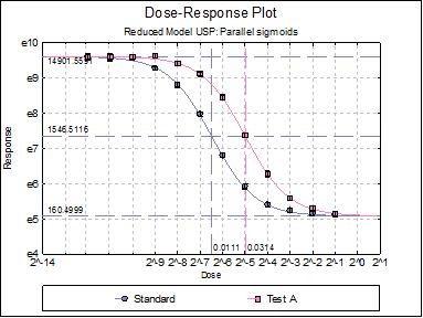
Click the Last Dialogue button to obtain the Output Options Dialogue and click [Back]. Select Reduced Model: Fit parallel sigmoids on selected preparations. On the next dialogue check only Test A, as it is the only test preparation meeting the selection criteria. Leave output options unchanged and then click [Finish].
Four-Parameter Logistic Model
Valid Number of Cases: 192, 192 Omitted
Model selected: Reduced Model USP
Regression Results
|
|
Coefficient |
Standard Error |
t-Statistic |
2-Tail Prob |
Lower 90% |
Upper 90% |
|
A |
14901.5591 |
444.0137 |
33.5610 |
0.0000 |
13997.7665 |
15805.3517 |
|
D |
160.4999 |
6.2979 |
25.4846 |
0.0000 |
147.6804 |
173.3193 |
|
B |
-1.4941 |
0.0551 |
-27.1126 |
0.0000 |
-1.6063 |
-1.3820 |
|
Standard EC50 |
0.0111 |
0.0004 |
29.9367 |
0.0000 |
0.0104 |
0.0119 |
|
Test A EC50 |
0.0314 |
0.0010 |
30.0153 |
0.0000 |
0.0293 |
0.0336 |
|
Total Residual Variance = |
0.0440 |
|
Degrees of Freedom = |
187 |
|
Satterthwaite DoF = |
4.7821 |
Correlation Matrix of Regression Coefficients
|
|
A |
D |
B |
Standard EC50 |
Test A EC50 |
|
A |
1.0000 |
-0.2272 |
-0.5248 |
-0.2760 |
-0.2792 |
|
D |
-0.2272 |
1.0000 |
0.6047 |
-0.4291 |
-0.4232 |
|
B |
-0.5248 |
0.6047 |
1.0000 |
-0.1069 |
-0.1030 |
|
Standard EC50 |
-0.2760 |
-0.4291 |
-0.1069 |
1.0000 |
0.3294 |
|
Test A EC50 |
-0.2792 |
-0.4232 |
-0.1030 |
0.3294 |
1.0000 |
Case (Diagnostic) Statistics
|
|
LogE(Response) |
Dose |
Preparation |
Plate |
Estimated Response |
95% lb Actual Y |
95% lb Mean of Y |
|
** 1 |
4.5962 |
0.5000 |
Standard |
Plate 1 |
5.0936 |
1.9426 |
4.5478 |
|
2 |
4.9461 |
0.5000 |
Standard |
Plate 1 |
5.0936 |
1.9426 |
4.5478 |
|
3 |
5.2660 |
0.5000 |
Standard |
Plate 2 |
5.0936 |
1.9426 |
4.5478 |
|
4 |
5.1606 |
0.5000 |
Standard |
Plate 2 |
5.0936 |
1.9426 |
4.5478 |
|
5 |
5.2318 |
0.5000 |
Standard |
Plate 3 |
5.0936 |
1.9426 |
4.5478 |
|
… |
… |
… |
… |
… |
|
|
… |
|
|
95% ub Mean of Y |
95% ub Actual Y |
Residuals |
Standardised Residuals |
Studentised Residuals |
|
** 1 |
5.6395 |
8.2446 |
-0.4974 |
-2.3705 |
-0.5053 |
|
2 |
5.6395 |
8.2446 |
-0.1475 |
-0.7030 |
-0.1498 |
|
3 |
5.6395 |
8.2446 |
0.1723 |
0.8214 |
0.1751 |
|
4 |
5.6395 |
8.2446 |
0.0669 |
0.3190 |
0.0680 |
|
5 |
5.6395 |
8.2446 |
0.1381 |
0.6583 |
0.1403 |
|
… |
… |
… |
… |
… |
… |
Cases marked by ‘**’ are outliers at 2 x Standard Deviation.
Effective Dose
|
|
Dose |
Standard Error |
Lower 90% |
Upper 90% |
|
Standard ED10 |
0.0026 |
0.0002 |
0.0022 |
0.0029 |
|
ED20 |
0.0044 |
0.0002 |
0.0040 |
0.0048 |
|
ED50 |
0.0111 |
0.0004 |
0.0104 |
0.0119 |
|
ED80 |
0.0281 |
0.0014 |
0.0253 |
0.0310 |
|
ED90 |
0.0484 |
0.0032 |
0.0419 |
0.0550 |
|
Test A ED10 |
0.0072 |
0.0004 |
0.0063 |
0.0081 |
|
ED20 |
0.0124 |
0.0006 |
0.0113 |
0.0136 |
|
ED50 |
0.0314 |
0.0010 |
0.0293 |
0.0336 |
|
ED80 |
0.0795 |
0.0040 |
0.0714 |
0.0877 |
|
ED90 |
0.1368 |
0.0091 |
0.1183 |
0.1554 |
Validity of Assay
|
Due To |
Sum of Squares |
DoF |
Mean Square |
F-Stat |
Prob |
|
Preparations |
25.144 |
3 |
8.381 |
245.449 |
0.0000 |
|
Regression |
1266.637 |
3 |
422.212 |
12364.460 |
0.0000 |
|
Non-parallelism |
0.013 |
3 |
0.004 |
0.124 |
0.9460 |
|
Non-linearity |
0.000 |
38 |
0.000 |
0.000 |
1.0000 |
|
Treatments |
1287.181 |
47 |
27.387 |
802.021 |
0.0000 |
|
Plate |
5.019 |
3 |
1.673 |
48.993 |
0.0000 |
|
Residual |
11.371 |
333 |
0.034 |
|
|
|
Total |
1300.756 |
383 |
3.396 |
|
|
|
R-squared |
0.991 |
|
|
|
|
ANOVA of Regression
|
Due To |
Sum of Squares |
DoF |
Mean Square |
F-Stat |
Prob |
|
Regression |
654.740 |
4 |
163.685 |
4514.212 |
0.0000 |
|
Error |
6.781 |
187 |
0.036 |
|
|
|
Total |
661.520 |
191 |
3.463 |
|
|
|
R-squared |
0.990 |
|
|
|
|
Measures of Variability
|
|
Standard Deviation |
Upper 95% Standard Deviation |
Upper 95% GSD |
Upper 95% %GCV |
Upper 95% %CV |
|
Within Plate |
0.0968 |
0.1058 |
1.1116 |
11.1636 |
10.6130 |
|
Between Plate |
0.1862 |
|
|
|
|
|
Total |
0.2098 |
0.5535 |
1.7393 |
73.9327 |
59.8725 |
Potency
|
|
Estimated Potency |
Lower 95% |
Upper 95% |
|
Test A |
2.8258 |
2.5551 |
3.1251 |
|
|
Relative Potency |
Lower 95% |
Upper 95% |
|
Test A |
282.58% |
255.51% |
312.51% |
|
|
Percent CI |
Lower 95% |
Upper 95% |
|
Test A |
100.00% |
90.42% |
110.59% |
