10.0. Overview
In cases where effectivity of a drug or a substance cannot be assessed by chemical or physical analysis, it can be assessed by testing its effects on biological organisms. Such experiments are called biological assays, or bioassays in short. The most common form of bioassay is where the potency of one or more test preparations is determined by comparison to a standard preparation.
This module supports potency calculations employing Parallel Line Method, Slope Ratio Method, Quantal Response Method, Four-Parameter Logistic Model and some Specific Assays, complete with confidence intervals, validity tests, predictions and graphical representations. Note that other types of bioassays and effective dose (or ED50) applications can be analysed using UNISTAT’s Nonlinear Regression procedure.
10.0.1. Data Preparation
Bioassay data is usually given in the form of a table where response measurements corresponding to different preparations and treatment groups are shown in separate columns. Additional information such as dose ratio and pre-dilutions / reconstitutions may be provided separately.
Example 1
Consider the following hypothetical 3-dose / 2-preparation Parallel Line Method example with 4 replicates, where the dose ratio is given as 1:2.
|
|
Preparations |
|||||
|
|
Standard |
Test |
||||
|
Replicates |
Dose 1 |
Dose 2 |
Dose 3 |
Dose 1 |
Dose 2 |
Dose 3 |
|
1 |
1.3 |
2.1 |
4.1 |
1.5 |
2.0 |
3.9 |
|
2 |
1.7 |
2.3 |
4.2 |
1.1 |
1.9 |
4.6 |
|
3 |
1.1 |
2.7 |
3.9 |
0.9 |
2.1 |
4.0 |
|
4 |
1.5 |
2.2 |
4.3 |
1.0 |
2.2 |
3.7 |
Although this is a well-defined and balanced data set for a bioassay, it should be first transformed into a more convenient format for analysis using a statistical package. This is done by stacking all response measurements in a single column. It is also necessary to create a number of categorical data columns (or factors) to keep track of which measurement belongs to which preparation, to which dose group and to which treatment case.
For analysis with UNISTAT, the data for the above example should be entered in a format similar to a database table, as follows:
|
Data |
Dose Ratio |
Preparation |
Rows |
Columns |
|
1.3 |
1 |
Standard |
1 |
1 |
|
1.7 |
1 |
Standard |
2 |
1 |
|
1.1 |
1 |
Standard |
3 |
1 |
|
1.5 |
1 |
Standard |
4 |
1 |
|
2.1 |
2 |
Standard |
1 |
2 |
|
2.3 |
2 |
Standard |
2 |
2 |
|
2.7 |
2 |
Standard |
3 |
2 |
|
2.2 |
2 |
Standard |
4 |
2 |
|
4.1 |
4 |
Standard |
1 |
3 |
|
4.2 |
4 |
Standard |
2 |
3 |
|
3.9 |
4 |
Standard |
3 |
3 |
|
4.3 |
4 |
Standard |
4 |
3 |
|
1.5 |
1 |
Test |
1 |
1 |
|
1.1 |
1 |
Test |
2 |
1 |
|
0.9 |
1 |
Test |
3 |
1 |
|
1.0 |
1 |
Test |
4 |
1 |
|
2.0 |
2 |
Test |
1 |
2 |
|
1.9 |
2 |
Test |
2 |
2 |
|
2.1 |
2 |
Test |
3 |
2 |
|
2.2 |
2 |
Test |
4 |
2 |
|
3.9 |
4 |
Test |
1 |
3 |
|
4.6 |
4 |
Test |
2 |
3 |
|
4.0 |
4 |
Test |
3 |
3 |
|
3.7 |
4 |
Test |
4 |
3 |
The first five characters of the standard preparation label should be “stand” or “refer” in any language (capitalisation is not significant). Otherwise the first preparation encountered in the [Preparation] column will be considered as the standard.
The Dose column may contain the dose ratios or actual dose units. Also, the column Rows is needed for Randomised Block, Latin Square Design and Crossover Design and Columns is needed for Latin Square Design and Crossover Design. In Stand-Alone Mode, Rows and Columns variables can be generated automatically by using UNISTAT spreadsheet functions Level(4) and Level(4);B respectively (see 3.4.2.5. Statistical Functions).
Example 2
The above example is nice and balanced and it may not be obvious why we need to transform the data to a database format after all. Consider though, the data for Quantal Response Method given in Table 18.2.1. on p. 376 Finney, D. J. (1978), an unbalanced assay with one test preparation.
|
Response |
Subject |
Dose IU/ml |
Preparation |
|
0 |
33 |
3.4 |
Standard |
|
5 |
32 |
5.2 |
Standard |
|
11 |
38 |
7 |
Standard |
|
14 |
37 |
8.5 |
Standard |
|
18 |
40 |
10.5 |
Standard |
|
21 |
37 |
13 |
Standard |
|
23 |
31 |
18 |
Standard |
|
30 |
37 |
21 |
Standard |
|
27 |
30 |
28 |
Standard |
|
2 |
40 |
6.5 |
Unknown |
|
10 |
30 |
10 |
Unknown |
|
18 |
40 |
14 |
Unknown |
|
21 |
35 |
21.5 |
Unknown |
|
27 |
37 |
29 |
Unknown |
The database format is the most natural way of representing the bioassay data.
10.0.2. Doses, Dilutions and Potency
When analysing bioassay data using one of four bioassay methods (Parallel Line Method, Slope Ratio Method, Quantal Response Method and Four-Parameter Logistic Model), if the actual dose levels administered are given (as in Example 2 above), we will readily obtain the estimated potency and its confidence limits in the same dose units.
However, dose data is often given as a ratio such as 1:2 or 5:4, where successive dose levels are calculated as multiples of this ratio starting or ending with 1 (as in Example 1 above). We call this kind of unitless dose data relative dose levels. Running a bioassay analysis on such data, one obtains a unitless relative potency (or potency ratio) with its confidence limits.
The optional [Dilution] data variable allows the user to enter all necessary potency and pre-dilution information (such as assigned potency of the standard, assumed potency of each test preparation and pre-dilutions for all preparations including the standard) and UNISTAT will calculate the estimated potency using this data. Here we use the term pre-dilution to include reconstitutions, unit transformations, volume administrations, conversions and inoculations.
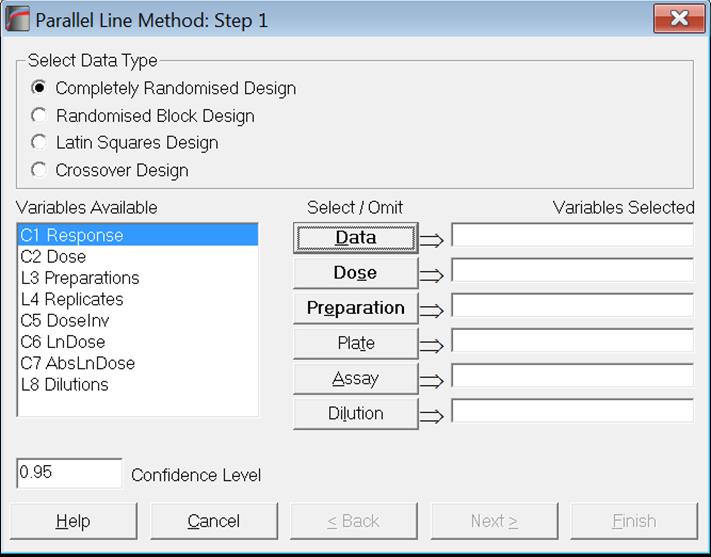
The optional [Dilution] data variable is common to all four bioassay methods Parallel Line Method, Slope Ratio Method, Quantal Response Method and Four-Parameter Logistic Model. It is expected to be a long string column (see 3.0.2.2.2. Long Strings) adhering strictly to the following format:
Row 1: Assigned potency of Standard
Row 2: All pre-dilutions of Standard separated by semicolons
Row 3: Assumed potency of Sample 1
Row 4: All pre-dilutions of Sample 1 separated by semicolons
Row 5: Assumed potency of Sample 2 (if any)
Row 6: All pre-dilution of Sample 2 separated by semicolons (if any)
…
Potencies and pre-dilutions can be entered as numbers followed by their units. Units are optional and spaces are not significant. If there is no information available for an item it should be entered as unity “1” or the cell can be left blank. This would be a typical example for a one-sample assay:
10345 IU/ampoule
1 ampoule / 50 ml; 1 ml / 10 ml
1
25.4 mg / 25 ml; 1 ml / 40 ml
If a [Dilution] data variable is not selected, all preparations are assumed to have a potency of 1 (unity) and a pre-dilution of 1, in which case the estimated potency is the relative potency or the potency ratio.
Following European Pharmacopoeia (1997-2017), UNISTAT applies the following rules in calculating the estimated potency.
Case 1: Standard and test preparations are not equipotent
UNISTAT runs a simple check to see if all pre-dilution values are entered as unity. If they are not, it concludes that the standard and test preparations are not equipotent and makes the following calculation to obtain the estimated potency and its confidence limits:
estimated potency of sample i = relative potency of sample i *
assigned potency of standard *
(pre-dilution of standard / pre-dilution of sample i).
Note that in this case the assumed potency of a test preparation does not play a role in potency calculations.
Case 2: Standard and test preparations are equipotent
If all pre-dilution values are entered as unity then UNISTAT concludes that the standard and test preparations are equipotent. In this case there are two further possibilities:
Case 2a: Assumed potency of test preparation is given (or not unity)
estimated potency of sample i = relative potency of sample i *
assumed potency of sample i
Case 2b: Assumed potency of test preparation is not given (or unity)
estimated potency of sample i = relative potency of sample i *
assigned potency of standard.
10.0.3. Potency Calculation Example
If the data column [Dose] contains the actual dose levels administered in original dose units, we will obtain the estimated potency and its confidence limits in the same units. If, however, the [Dose] column contains unitless relative dose levels, then the reported estimated potency will be the unitless relative potency or the potency ratio. Then, we may need to perform further calculations to obtain the estimated potency in original potency units.
Consider the following 2-preparation, 3-dose, 4-replicate balanced assay of kanamycin monosulfate where the dose ratio is given as 3:2.
|
Standard |
||||
|
Id. |
Kanamycin monosulfate WHO 1st IS |
|||
|
Assigned potency |
10345 IU/ampoule |
|||
|
Reconstituition |
1 ampoule/50mL |
|||
|
Pre-dilution 1 |
1mL/10mL |
|||
|
Doses |
(1) |
(2) |
(3) |
(4) |
|
S1 |
20.0 |
20.4 |
20.9 |
20.7 |
|
S2 |
21.7 |
22.0 |
22.0 |
21.5 |
|
S3 |
22.4 |
23.0 |
23.5 |
23.0 |
|
Sample 1 |
||||
|
Id. |
Kanamycin monosulfate CRS3 |
|||
|
Assumed potency |
? IU/mg |
|||
|
Reconstituition |
25.40 mg/25mL |
|||
|
Pre-dilution 1 |
1mL/40mL |
|||
|
Doses |
(1) |
(2) |
(3) |
(4) |
|
T1 |
20.0 |
20.4 |
20.4 |
20.2 |
|
T2 |
21.5 |
21.7 |
21.9 |
22.0 |
|
T3 |
22.8 |
23.3 |
23.3 |
23.2 |
Using UNISTAT, we can estimate the potency of Sample 1 with one of the following two methods.
10.0.3.1. Dose Ratio and Pre-dilutions are Given
Using the data transformation described in section 10.0.1. Data Preparation these two tables can be represented in database format as follows:
|
Data |
Dose |
Preparation |
Replicate |
Dilution |
|
20 |
1 |
Standard |
1 |
10345IU/ampoule |
|
20.4 |
1 |
Standard |
2 |
1ampoule/50ml;1ml/10ml |
|
20.9 |
1 |
Standard |
3 |
1 |
|
20.7 |
1 |
Standard |
4 |
25.4mg/25ml;1ml/40ml |
|
21.7 |
1.5 |
Standard |
1 |
|
|
22 |
1.5 |
Standard |
2 |
|
|
22 |
1.5 |
Standard |
3 |
|
|
21.5 |
1.5 |
Standard |
4 |
|
|
22.4 |
2.25 |
Standard |
1 |
|
|
23 |
2.25 |
Standard |
2 |
|
|
23.5 |
2.25 |
Standard |
3 |
|
|
23 |
2.25 |
Standard |
4 |
|
|
20 |
1 |
Sample 1 |
1 |
|
|
20.4 |
1 |
Sample 1 |
2 |
|
|
20.4 |
1 |
Sample 1 |
3 |
|
|
20.2 |
1 |
Sample 1 |
4 |
|
|
21.5 |
1.5 |
Sample 1 |
1 |
|
|
21.7 |
1.5 |
Sample 1 |
2 |
|
|
21.9 |
1.5 |
Sample 1 |
3 |
|
|
22 |
1.5 |
Sample 1 |
4 |
|
|
22.8 |
2.25 |
Sample 1 |
1 |
|
|
23.3 |
2.25 |
Sample 1 |
2 |
|
|
23.3 |
2.25 |
Sample 1 |
3 |
|
|
23.2 |
2.25 |
Sample 1 |
4 |
|
Let us now analyse this data with Parallel Line Method and selecting the Randomised Block Design.
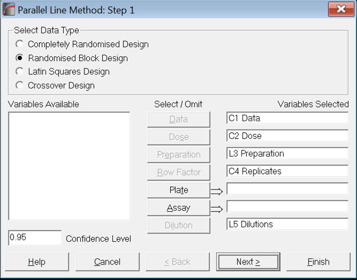
Click [Next] to display the Output Options Dialogue, click None to uncheck all options and then check the Potency option.
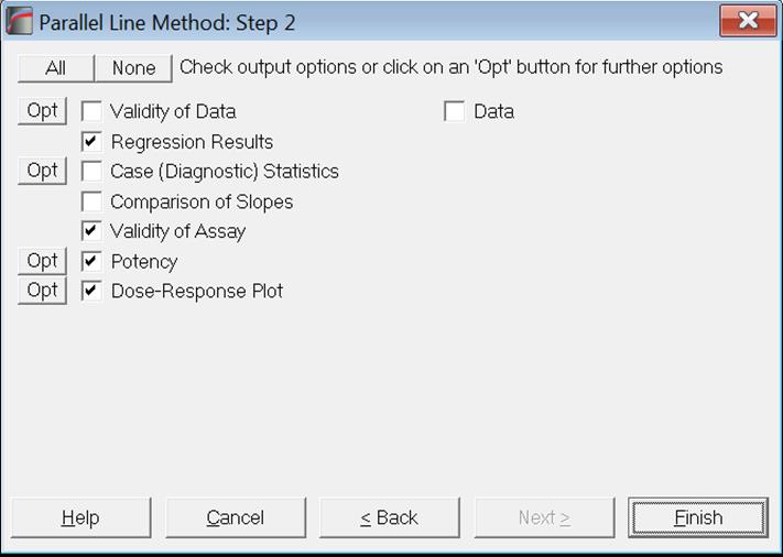
Clicking [Finish], the following results are obtained:
Parallel Line Method
Potency
Randomised Block Design
Assigned potency of Standard: 10345IU/ampoule
Pre-dilution of Standard: 1ampoule/50ml;1ml/10ml
Pre-dilution of Sample 1: 25.4mg/25ml;1ml/40ml
|
|
Estimated Potency |
Lower 95% |
Upper 95% |
DoF |
% Precision |
|
Sample 1 |
806.4150 |
766.7124 |
848.0747 |
15 |
95.08% |
|
|
Relative Potency |
Lower 95% |
Upper 95% |
|
Sample 1 |
99.00% |
94.13% |
104.11% |
|
|
Percent CI |
Lower 95% |
Upper 95% |
|
Sample 1 |
100.00% |
95.08% |
105.17% |
|
G = |
0.0058 |
|
C = |
1.0058 |
Note that only those potency or pre-dilution values that are different from unity are reported in the output.
As the standard and sample are not equipotent, UNISTAT makes the following calculation to obtain the estimated potency and its confidence limits:
estimated potency of sample i = relative potency of sample i *
assigned potency of standard *
(pre-dilution of standard / pre-dilution of sample i).
10.0.3.2. Actual Dose Levels are Given
Alternatively, we can calculate the actual dose levels from the dose ratio and the given pre-dilutions of standard and sample as:
Actual dose of standard = relative dose of standard *
assigned potency of standard *
pre-dilution of standard.
and:
Actual dose of sample i = relative dose of sample i *
pre-dilution of sample i.
For the example in previous section, the actual dose values are calculated for Standard as:
1 * 10345 * (1/50)*(1/10) = 20.69 IU/mL
1.5 * 10345 * (1/50)*(1/10) = 31.035 IU/mL
2.25 * 10345 * (1/50)*(1/10) = 46.5525 IU/mL
and for Sample 1 as:
1 * (25.4/25)*(1/40) = 0.0254 IU/mL
1.5 * (25.4/25)*(1/40) = 0.0381 IU/mL
2.25 * (25.4/25)*(1/40) = 0.05715 IU/mL
The data table to analyse will therefore be as follows:
|
Data |
Dose IU/mL |
Preparation |
Replicate |
|
20 |
20.69 |
Standard |
1 |
|
20.4 |
20.69 |
Standard |
2 |
|
20.9 |
20.69 |
Standard |
3 |
|
20.7 |
20.69 |
Standard |
4 |
|
21.7 |
31.035 |
Standard |
1 |
|
22 |
31.035 |
Standard |
2 |
|
22 |
31.035 |
Standard |
3 |
|
21.5 |
31.035 |
Standard |
4 |
|
22.4 |
46.5525 |
Standard |
1 |
|
23 |
46.5525 |
Standard |
2 |
|
23.5 |
46.5525 |
Standard |
3 |
|
23 |
46.5525 |
Standard |
4 |
|
20 |
0.0254 |
Sample 1 |
1 |
|
20.4 |
0.0254 |
Sample 1 |
2 |
|
20.4 |
0.0254 |
Sample 1 |
3 |
|
20.2 |
0.0254 |
Sample 1 |
4 |
|
21.5 |
0.0381 |
Sample 1 |
1 |
|
21.7 |
0.0381 |
Sample 1 |
2 |
|
21.9 |
0.0381 |
Sample 1 |
3 |
|
22 |
0.0381 |
Sample 1 |
4 |
|
22.8 |
0.05715 |
Sample 1 |
1 |
|
23.3 |
0.05715 |
Sample 1 |
2 |
|
23.3 |
0.05715 |
Sample 1 |
3 |
|
23.2 |
0.05715 |
Sample 1 |
4 |
Again, running the Parallel Line Method with Randomised Block Design, and without selecting the [Dilution] variable, we obtain exactly the same results as in the previous section:
Parallel Line Method
Potency
Randomised Block Design
|
|
Estimated Potency |
Lower 95% |
Upper 95% |
|
Sample 1 |
806.4150 |
766.7124 |
848.0747 |
10.0.4. Multiple Assays with Combination
The optional variable type [Assay] is common to all bioassay analysis methods Parallel Line Method, Slope Ratio Method, Quantal Response Method, Four-Parameter Logistic Model and some Specific Assays. This variable makes it possible to run multiple assays and to combine their results in one go.
The format of multiple assay data is exactly the same as their former single assay versions, except that multiple assay data are stacked in the same columns and a new variable [Assay] (containing assay numbers or strings) is created to keep track of different assays.
Due to the complexity of multi-assay runs, the program will not stop for any intermediary dialogues. Output will be created right after clicking [Next] or [Finish] in the Variable Selection Dialogue. Previous selections made in any subsequent dialogues will be effective. Normally, arithmetic means of potencies should be calculated for Slope Ratio Method and geometric means for Parallel Line Method, Quantal Response Method and Four-Parameter Logistic Model. However, there may be exceptions for this. The user should ensure that the correct averaging method was selected in Combined Potency Output Options dialogue prior to running a multi-assay task.
Output consists of results for each assay followed by the combination of estimated potency results, as described in section 10.5. Combination of Assays.
Let us illustrate this with three 5+1 assays. Data with corrected means is given as follows.
|
Response |
Dose IU |
Preparation |
Assay |
Dilution |
|
15.17611 |
6.3989 |
Standard |
No 13267 |
1020 IU/mg |
|
15.49833 |
7.9937 |
Standard |
No 13267 |
1 |
|
16.13389 |
10 |
Standard |
No 13267 |
1020 IU/mg |
|
16.58278 |
12.5068 |
Standard |
No 13267 |
1 |
|
16.70611 |
15.6388 |
Standard |
No 13267 |
* |
|
16.07056 |
10 |
Test |
No 13267 |
* |
|
15.61806 |
6.3989 |
Standard |
No 13268 |
1020 IU/mg |
|
15.81806 |
7.9937 |
Standard |
No 13268 |
1 |
|
16.52917 |
10 |
Standard |
No 13268 |
1020 IU/mg |
|
17.13806 |
12.5068 |
Standard |
No 13268 |
1 |
|
17.51472 |
15.6388 |
Standard |
No 13268 |
* |
|
16.51694 |
10 |
Test |
No 13268 |
* |
|
12.06028 |
6.3989 |
Standard |
No 13269 |
1020 IU/mg |
|
12.61694 |
7.9937 |
Standard |
No 13269 |
1 |
|
13.29361 |
10 |
Standard |
No 13269 |
1020 IU/mg |
|
13.77917 |
12.5068 |
Standard |
No 13269 |
1 |
|
14.28028 |
15.6388 |
Standard |
No 13269 |
|
|
13.19583 |
10 |
Test |
No 13269 |
|
Selecting variables as:
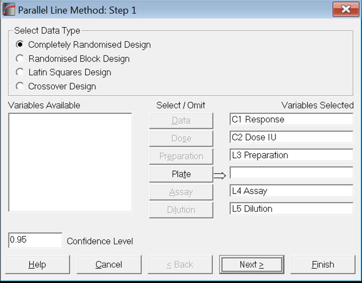
and clicking [Next] or [Finish] the following output is obtained. No further dialogues are displayed. Output options used in previous runs will be effective.
Parallel Line Method
Assay: No 13267
Completely Randomised Design
Validity of Assay
|
Due To |
Sum of Squares |
DoF |
Mean Square |
F-Stat |
Prob |
|
Preparations |
0.002 |
1 |
0.002 |
0.098 |
0.7752 |
|
Linear Regression |
1.718 |
1 |
1.718 |
77.000 |
0.0031 |
|
Non-linearity |
0.067 |
3 |
0.022 |
|
|
|
Standard Non-linearity |
0.067 |
3 |
0.022 |
|
|
|
Test Non-linearity |
0.000 |
0 |
|
|
|
|
Treatments |
1.787 |
5 |
0.357 |
|
|
|
Residual |
0.000 |
0 |
|
|
|
|
Total |
1.787 |
5 |
0.357 |
|
|
Potency
0 residual SSQ and DoF replaced by non-linearity SSQ and DoF.
Assigned potency of Standard: 1020 IU/mg
Assumed potency of Test: 1020 IU/mg
|
|
Estimated Potency |
Lower 95% |
Upper 95% |
|
Test |
1048.6031 |
778.8981 |
1423.5329 |
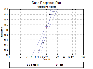
Parallel Line Method
Assay: No 13268
Completely Randomised Design
Validity of Assay
|
Due To |
Sum of Squares |
DoF |
Mean Square |
F-Stat |
Prob |
|
Preparations |
0.000 |
1 |
0.000 |
0.002 |
0.9689 |
|
Linear Regression |
2.615 |
1 |
2.615 |
125.815 |
0.0015 |
|
Non-linearity |
0.062 |
3 |
0.021 |
|
|
|
Standard Non-linearity |
0.062 |
3 |
0.021 |
|
|
|
Test Non-linearity |
0.000 |
0 |
|
|
|
|
Treatments |
2.678 |
5 |
0.536 |
|
|
|
Residual |
0.000 |
0 |
|
|
|
|
Total |
2.678 |
5 |
0.536 |
|
|
Potency
0 residual SSQ and DoF replaced by non-linearity SSQ and DoF.
Assigned potency of Standard: 1020 IU/mg
Assumed potency of Test: 1020 IU/mg
|
|
Estimated Potency |
Lower 95% |
Upper 95% |
|
Test |
1017.1244 |
808.6856 |
1278.6352 |
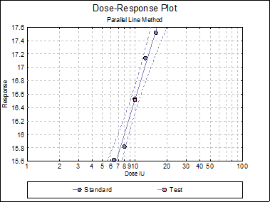
Parallel Line Method
Assay: No 13269
Completely Randomised Design
Validity of Assay
|
Due To |
Sum of Squares |
DoF |
Mean Square |
F-Stat |
Prob |
|
Preparations |
0.000 |
1 |
0.000 |
0.023 |
0.8896 |
|
Linear Regression |
3.138 |
1 |
3.138 |
820.057 |
0.0001 |
|
Non-linearity |
0.011 |
3 |
0.004 |
|
|
|
Standard Non-linearity |
0.011 |
3 |
0.004 |
|
|
|
Test Non-linearity |
0.000 |
0 |
|
|
|
|
Treatments |
3.150 |
5 |
0.630 |
|
|
|
Residual |
0.000 |
0 |
|
|
|
|
Total |
3.150 |
5 |
0.630 |
|
|
Potency
0 residual SSQ and DoF replaced by non-linearity SSQ and DoF.
Assigned potency of Standard: 1020 IU/mg
Assumed potency of Test: 1020 IU/mg
|
|
Estimated Potency |
Lower 95% |
Upper 95% |
|
Test |
1015.9423 |
931.6402 |
1107.7597 |
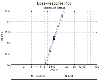
Combination of Assays
Homogeneity Tests
|
|
Chi-Square |
DoF |
Probability |
|
Mean |
0.1033 |
2 |
0.9497 |
|
Variance |
3.3161 |
2 |
0.1905 |
Combined Potency EP
|
Geometric Mean |
Potency |
Lower 95% |
Upper 95% |
|
Weighted EP |
1018.2457 |
963.1818 |
1076.4577 |
|
Semi-weighted EP |
1018.4889 |
966.8818 |
1072.8505 |
|
Unweighted |
1027.1127 |
982.3380 |
1073.9281 |
Combined Potency USP
|
Geometric Mean |
Potency |
Lower 95% |
Upper 95% |
|
Weighted USP |
1018.2457 |
922.0896 |
1124.4291 |
|
Semi-weighted USP |
1018.9299 |
955.3052 |
1086.7922 |
|
Unweighted |
1027.1127 |
982.3380 |
1073.9281 |
|
Standard Deviation (Log base e) = |
0.0179 |
|
Unweighted Mean (Log base e) = |
6.9345 |
|
%RSD = |
0.26% |
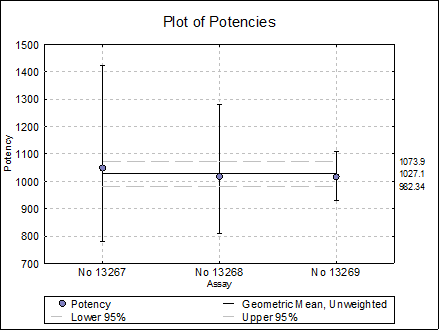
10.0.5. Compliance Options
UNISTAT provides a comprehensive set of tools (under Tools → Compliance menu option) to ensure its bioassay analysis procedures generate a publication quality report that complies with FDA 21 CFR Part 11 requirements. This menu item is enabled only when the optional Analysis of Bioassays module is activated and the user is granted Supervisor rights by a Windows system Administrator.
Many of the options are designed to work with Microsoft Word or Excel. For further information see section 2.4.1.2. Output. Note that you can also change the size of graphics objects in the output. See section 2.4.1.2.5. Graphics Size.
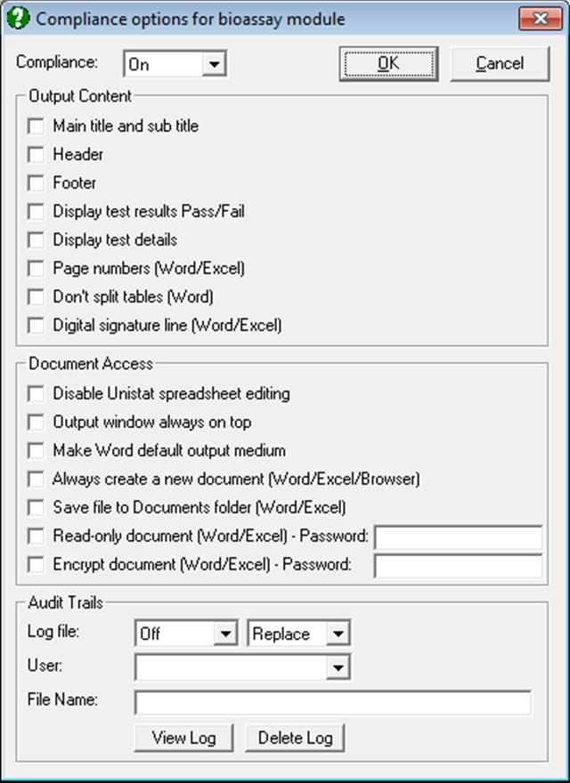
User access control
UNISTAT retrieves user access rights from the Windows system. User name and password are the user name and password entered to log in to the Windows system. If a user has full read/write control to this folder and all its subfolders:
C:\ProgramData\Unistat
then he or she will have access to the Compliance dialogue. Such a user is called a Supervisor. For a Standard User (or the Operator) the Tools → Compliance menu option will be disabled. A Supervisor can be a Windows system Administrator or a Standard User who is granted full read/write access to the above folder by a system Administrator.
The Supervisor can control the following options.
10.0.5.1. Compliance Output
Main title and sub title
It is possible to display a user-defined Main Title and a Sub Title for the whole document. The Main Title text will be retrieved from Row Label 1 and the Sub Title text from Row Label 2. For further information see sections 3.2.11. Row Labels and 2.4.1.6.2. Labels.
Header
Headers and footers have a fixed first line which shows the program name and version.
|
UNISTAT Bioassay Analysis |
Version 10.11 |
|
User: unist |
Role: Supervisor |
|
Date: 06/05/2020 19:41:11 |
File: EP541 |
When Row Labels 3, 4, 5 and 6 are blank, the next two lines of the header table is generated by the program with the following four cells:
User: The user name is the current user’s Windows login ID and it is retrieved from the Windows environment by the program.
Role: Can be Supervisor or Operator and it is retrieved from the Windows environment by the program.
Date: Windows system date and time.
File: In Stand-Alone Mode this is the name of the file currently open in UNISTAT spreadsheet (without a file extension). In Excel Add-In Mode the file name is fixed as ComplianceDoc.
Any text entered into Row Labels 3, 4, 5 and 6 will replace the corresponding default header text. It is possible to add further items to the header by entering text into row label 7 onwards. UNISTAT will extend the table accordingly.
Footer
The header table can also be displayed at the end of the document, before the signature line. By default, only the first three lines of the header are duplicated by the program, but it is possible to display a footer identical to header by entering the following line:
FooterLikeHeader=1
under the [Bioassay] section of the following file:
C:\ProgramData\Unistat\Unistat10\Unistat10.ini
Display test results Pass/Fail
UNISTAT normally reports result of hypothesis testing as a probability value which the user is expected to compare with a pre-determined threshold (usually 5%) to determine whether the test result is a Pass or Fail. When this option is checked, UNISTAT will add a further column to the output table indicating a Pass or Fail test result.
Validity of Assay
|
Due To |
Sum of Squares |
DoF |
Mean Square |
F-Stat |
Prob |
Pass/Fail |
|
Preparations |
4.475 |
3 |
1.492 |
223.395 |
0.0000 |
Pass |
|
Linear Regression |
47.584 |
1 |
47.584 |
7125.912 |
0.0000 |
Pass |
|
Non-parallelism |
0.019 |
3 |
0.006 |
0.933 |
0.4339 |
Pass |
|
Non-linearity |
0.074 |
12 |
0.006 |
0.926 |
0.5307 |
Pass |
|
Standard S Non-linearity |
0.017 |
3 |
0.006 |
0.850 |
0.4747 |
Pass |
|
Preparation T Non-linearity |
0.028 |
3 |
0.009 |
1.410 |
0.2538 |
Pass |
|
Preparation U Non-linearity |
0.018 |
3 |
0.006 |
0.886 |
0.4564 |
Pass |
|
Preparation V Non-linearity |
0.011 |
3 |
0.004 |
0.559 |
0.6455 |
Pass |
|
Treatments |
52.152 |
19 |
2.745 |
411.053 |
0.0000 |
Pass |
|
Residual |
0.267 |
40 |
0.007 |
|
|
|
|
Total |
52.419 |
59 |
0.888 |
|
|
|
Test results are reported for ANOVA tables, R-squared values and homogeneity and percent potency tests.
The default threshold probability and the inequality sign used in tests can be displayed and/or edited as described below.
Display test details
This option is only effective when the Display test results Pass/Fail option above is also checked. In this case a description line will be added below the table for each test, showing the name of the test, the test statistic, the inequality, the probability threshold used in the test and the test result Pass/Fail.
|
Treatments |
52.152 |
19 |
2.745 |
411.053 |
0.0000 |
Pass |
|
Residual |
0.267 |
40 |
0.007 |
|
|
|
|
Total |
52.419 |
59 |
0.888 |
|
|
|
ParallelPreparations: 5.16170046091974E-25 LT 0.05 Pass
ParallelRegression: 1.08423673494635E-46 LT 0.01 Pass
ParallelNonParallelism: 0.433876017762221 GT 0.05 Pass
ParallelNonLinearity: 0.530744876258032 GT 0.05 Pass
ParallelNonLinearity1: 0.474733337243044 GT 0.05 Pass
ParallelNonLinearity2: 0.253844569354657 GT 0.05 Pass
ParallelNonLinearity3: 0.45638906296038 GT 0.05 Pass
ParallelNonLinearity4: 0.645474480915028 GT 0.05 Pass
ParallelTreatments: 7.52607017266053E-40 LT 0.01 Pass
|
|
Percent CI |
Lower 95% |
Upper 95% |
Pass/Fail |
|
Preparation T |
100.00% |
93.38% |
107.19% |
Pass |
|
Preparation U |
100.00% |
93.48% |
107.05% |
Pass |
|
Preparation V |
100.00% |
93.43% |
107.12% |
Pass |
PotencyPctLower: 93.3789844253378 GT 75 Pass
AND
PotencyPctUpper: 107.185745855585 LT 125 Pass
PotencyPctLower: 93.4784832478474 GT 75 Pass
AND
PotencyPctUpper: 107.045754050987 LT 125 Pass
PotencyPctLower: 93.4288713117567 GT 75 Pass
AND
PotencyPctUpper: 107.116581482308 LT 125 Pass
The Supervisor can change the threshold probabilities by entering the name of the test as displayed here equal to a new threshold, under the [Bioassay] section of the following file:
C:\ProgramData\Unistat\Unistat10\Unistat10.ini
For instance, if the following line is added to this file:
ParallelPreparations=0.01
then only P-values less than 0.01 will generate a Pass for this test. Note that there should be only one [Bioassay] section in this file.
If you do not wish to display one of the test results, say the Treatments test, add the following line under the [Bioassay] section of the above file:
ParallelTreatments=-1
The Pass/Fail cell of the Treatments line of the table will appear blank.
Page numbers (Word/Excel)
Page numbers will be inserted at mid-bottom of each page in the format of Page I of J, where J is the total number of pages in the report.
Don’t split tables (Word)
When this option is checked, tables in Word output will not be split across the pages, as much as possible.
Digital signature line (Word/Excel)
Word and Excel report files can be digitally signed by the current user. Administration and allocation of digital signatures is the responsibility of the customer. UNISTAT will insert a signature line, and if the Save file to Documents folder option below is checked, it will save the document. The document can then be signed digitally by the current user.
Occasionally, this window may pop up when the signature line is inserted. In such cases click [OK] to continue.
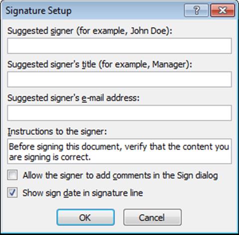
In Word 2010 or earlier versions, the following information line appears on top of the document:

Clicking the View signatures… button, a Signatures pane opens on the right. Right-click on the correct Requested signature and select Sign. The following dialogue pops up:
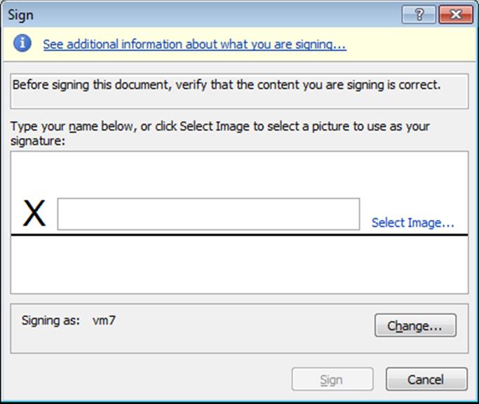
Either type a name or select a signature image and click Sign. The document will be signed and saved again.
In Word 2013 or later versions, the following information line appears on top of the document:

In this case you need to select VIEW and then select Edit document first, to be able to click on View signatures… button. This will not render the document editable, but will allow the user to sign the document.
10.0.5.2. Compliance Access
Disable Unistat spreadsheet editing
When using UNISTAT in Stand-Alone Mode, the Standard User can be prevented from making any changes to the data. When this box is checked, the Operator can only open files and perform procedures under the Bioassay menu option.
By default, this option will not disable the Bioassay and Tools menu options. If you wish, you can also disable these two menu items by entering the following line:
DisableBioTools=1
under the [Bioassay] section of this file:
C:\ProgramData\Unistat\Unistat10\Unistat10.ini
In this case the only way to run a procedure is through a user-defined macro button as described in section 2.4.2.4. Macro Shortcut Buttons.
Output window always on top
In some cases, the output (i.e. UNISTAT Output Window, Word or Excel) can remain behind other applications. When this option is checked, the output window will be forced to appear on the foreground.
Make Word default output medium
This is equivalent to setting the Default Output Medium to Word for Windows from Tools → Options dialogue’s Output tab.
Always create a new document (Word/Excel/Browser)
If this option is not checked, the output will be created as follows:
Word: If one or more Word documents are open, the output will be inserted into the current cursor location in the most recently activated document.
Excel: A new sheet will be inserted in the most recently activated workbook.
Browser: Output will be appended to this document:
..\Documents\Unistat10\HTML\Unistat.html
If this option is checked, the existing contents of this html file will be overwritten with the new output.
Save file to Documents folder (Word/Excel)
Output will be saved to the current user’s Documents folder. In Stand-Alone Mode the output file will have the name of the file currently open in UNISTAT spreadsheet. In Excel Add-In Mode the file name is fixed to ComplianceDoc. If a file with the same name and file extensions exists in the Documents folder, it will be overwritten without a further prompt.
If Word is the output medium, the active document will be saved and opened again. If Excel is the output medium then the entire workbook will be saved but will not be opened again.
As the inserted digital signature line cannot be signed without saving and opening a document, this option will enable the user to sign a Word document instantly. To sign an Excel file, it must be opened again manually.
Read-only document (Word/Excel) – Password
This is one of the basic requirements of compliance and should be checked in most cases. The Supervisor should enter a password not shorter than 8 characters and once this password is entered the document cannot be edited by any users. Note that this is independent of write-protection that comes with digitally signing the document. If you remove the signature the document still cannot be edited.
Encrypt document (Word/Excel) – Password
When this option is checked and a password is entered, the saved Word or Excel files cannot be opened without entering this password. As this will prevent a saved Word file to be opened automatically by the program, it must be used with caution.
10.0.5.3. Compliance Audit Trails
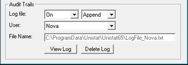
This option facilitates keeping a record of all selections made by each user from UNISTAT’s Bioassay menu. The spreadsheet operations are not logged.
Select log file On to record audit trails for all users. If the Append, option is selected the logs will be written to the same file and nothing in the log file will be deleted. If the Replace option is selected, the old log file will be deleted at the start of each session.
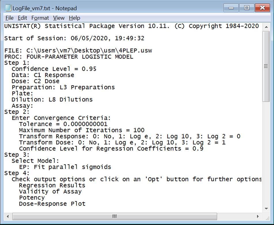
The User list will show which users have log files. The Supervisor can select a user name from the list and open his/her log file by clicking on the View Log button. The default location for log files is:
C:\ProgramData\Unistat\Unistat10
Note that when the Append option is on, the log files will keep on growing. It is the customer’s responsibility to maintain these files.
10.0.5.4. IQ OQ PQ
A comprehensive IQ/OQ/PQ (or IQ-OQ-PQ , IQOQPQ) package is available from Unistat Ltd (info@unistat.com) upon request. It contains the following sections:
· Installation Qualification (IQ) for Administrators and Standard Users,
· Operational Qualification (OQ) featuring a validation of Unistat’s numeric results against European Pharmacopoeia (1997-2017) and United States Pharmacopoeia (2010) and a fully automated target installation verification,
· Performance Qualification (PQ) tools enabling the customer to compile PQ documents with ease.
10.0.6. Outlier Detection, Omission and Replacement
United States Pharmacopoeia <111> (2010) and European Pharmacopoeia (1997-2017) require bioassay data to be checked for outliers. This can be done in two ways; first, by checking the raw data for outliers in treatment (i.e. unique dose-preparation) groups, where data points are expected to be roughly equal, and secondly, after fitting the model to data, finding out which response values deviate most from the values estimated by the model. UNISTAT provides powerful tools to detect outliers using both methods.
10.0.6.1. Outlier Detection in Treatment Groups
UNISTAT supports three commonly used outlier tests as part of bioassay analysis procedures; Dixon, Grubbs and ESD (Generalised Extreme Studentised Deviate). For more information see section 6.3.4. Outlier Tests.
Although all three detection methods can be run simultaneously, you are advised to select one of them depending on the data. For instance, Dixon’s test will probably be the best one when treatment group sizes are less than 15 and the Grubbs test may be better for group sizes greater than 25. While Dixon and Grubbs tests are used to detect one outlier in each treatment group, ESD test can be used to detect a number of outliers up to a user-defined maximum.
Outliers detected here can be omitted or replaced and the assay calculations repeated. For more information see following sections of this chapter.
Example
Open BIOPHARMA9 and select Bioassay → Parallel Line Method. From the Variable Selection Dialogue select the first option Completely Randomised Design and then select columns C5, C6 and L7 respectively as [Data], [Dose], and [Preparation] Click [Next] to proceed to Output Options Dialogue and click on the [Opt] button situated to the left of Validity of Data option. Uncheck all options except Outlier Tests and click [Finish].
Dixon’s Outlier Test
Alpha = 0.05
One-tailed tests
|
Dose x Preparations |
Dixon’s Q |
Table Q |
Pass/Fail |
|
1 x Standard S Q(Min) |
0.0625 |
0.5624 |
Pass |
|
Q(Max) |
0.1875 |
0.5624 |
Pass |
|
1 x Preparation T Q(Min) |
0.0000 |
0.5624 |
Pass |
|
Q(Max) |
0.1000 |
0.5624 |
Pass |
|
1.5 x Standard S Q(Min) |
0.0769 |
0.5624 |
Pass |
|
Q(Max) |
0.1538 |
0.5624 |
Pass |
|
1.5 x Preparation T Q(Min) |
0.3333 |
0.5624 |
Pass |
|
Q(Max) |
0.2083 |
0.5624 |
Pass |
|
2.25 x Standard S Q(Min) |
0.3571 |
0.5624 |
Pass |
|
Q(Max) |
0.2143 |
0.5624 |
Pass |
|
2.25 x Preparation T Q(Min) |
0.1000 |
0.5624 |
Pass |
|
Q(Max) |
0.3000 |
0.5624 |
Pass |
N = 6, Q(Min)=(X(2)-X(1))/(X(N)-X(1)), Q(Max)=(X(N)-X(N-1))/(X(N)-X(1))
Grubbs’ Outlier Test
Alpha = 0.05
One-tailed tests
|
Dose x Preparations |
Grubbs’ G |
Table G |
Pass/Fail |
|
1 x Standard S G(Min) |
1.3145 |
1.8221 |
Pass |
|
G(Max) |
1.1123 |
1.8221 |
Pass |
|
1 x Preparation T G(Min) |
1.0974 |
1.8221 |
Pass |
|
G(Max) |
1.0266 |
1.8221 |
Pass |
|
1.5 x Standard S G(Min) |
1.0266 |
1.8221 |
Pass |
|
G(Max) |
1.4000 |
1.8221 |
Pass |
|
1.5 x Preparation T G(Min) |
1.4620 |
1.8221 |
Pass |
|
G(Max) |
1.3081 |
1.8221 |
Pass |
|
2.25 x Standard S G(Min) |
1.5471 |
1.8221 |
Pass |
|
G(Max) |
1.3408 |
1.8221 |
Pass |
|
2.25 x Preparation T G(Min) |
0.8669 |
1.8221 |
Pass |
|
G(Max) |
1.6100 |
1.8221 |
Pass |
G = Maximum deviation from mean / Standard Deviation
ESD Outlier Test
Alpha = 0.05
Two-tailed test
Number of outliers to test (ESD) = 2
|
Dose x Preparations |
ESD Ri |
Table Ri |
Pass/Fail |
|
1 x Standard S (Min) 1 |
1.3145 |
1.8871 |
Pass |
|
1 x Standard S (Min) 2 |
1.6669 |
1.7150 |
Pass |
|
1 x Preparation T (Min) 1 |
1.0974 |
1.8871 |
Pass |
|
1 x Preparation T (Min) 2 |
1.3969 |
1.7150 |
Pass |
|
1.5 x Standard S (Max) 1 |
1.4000 |
1.8871 |
Pass |
|
1.5 x Standard S (Max) 2 |
1.6059 |
1.7150 |
Pass |
|
1.5 x Preparation T (Min) 1 |
1.4620 |
1.8871 |
Pass |
|
1.5 x Preparation T (Max) 2 |
1.3017 |
1.7150 |
Pass |
|
2.25 x Standard S (Min) 1 |
1.5471 |
1.8871 |
Pass |
|
2.25 x Standard S (Max) 2 |
1.4142 |
1.7150 |
Pass |
|
2.25 x Preparation T (Max) 1 |
1.6100 |
1.8871 |
Pass |
|
2.25 x Preparation T (Max) 2 |
1.7298 |
1.7150 |
**Fail** |
Ri = Generalised Extreme Studentised Deviate
|
Dose x Preparations |
Outlier Value |
|
2.25 x Preparation T |
199 |
Dixon and Grubbs tests show no significant outliers. ESD test reports the value 199 in treatment group 2.25 x Preparation T as a possible outlier at a 5% threshold. You may as well take no action about this possible outlier, as USP <111> recommends no action unless there is overwhelming evidence for an outlier.
10.0.6.2. Model-Based Outlier Detection
In addition to the tests provided in previous section, outliers can also be detected using the Case (Diagnostic) Statistics output option. See section 10.1.2.3. Case (Diagnostic) Statistics. Such tests are called model-based, because they tell us which response values deviate most from the values estimated by the model.
Example
When you run the example given in previous section, the Case (Diagnostic) Statistics and Potency output will be as follows. Only the first 10 cases (rows) are shown to save space.
Case (Diagnostic) Statistics
|
|
Response |
Dose |
Preparations |
Estimated Response |
Residuals |
Standardised Residuals |
|
1 |
161 |
1 |
Standard S |
157.7639 |
3.2361 |
0.5684 |
|
2 |
151 |
1 |
Preparation T |
156.6528 |
-5.6528 |
-0.9928 |
|
** 3 |
162 |
1.5 |
Preparation T |
175.4444 |
-13.4444 |
-2.3612 |
|
4 |
194 |
2.25 |
Standard S |
195.3472 |
-1.3472 |
-0.2366 |
|
5 |
176 |
1.5 |
Standard S |
176.5556 |
-0.5556 |
-0.0976 |
|
6 |
193 |
2.25 |
Preparation T |
194.2361 |
-1.2361 |
-0.2171 |
|
7 |
160 |
1 |
Preparation T |
156.6528 |
3.3472 |
0.5879 |
|
8 |
192 |
2.25 |
Preparation T |
194.2361 |
-2.2361 |
-0.3927 |
|
9 |
195 |
2.25 |
Standard S |
195.3472 |
-0.3472 |
-0.0610 |
|
10 |
184 |
1.5 |
Standard S |
176.5556 |
7.4444 |
1.3075 |
|
… |
… |
… |
… |
… |
… |
… |
Cases marked by ‘**’ are outliers at 2 x Standard Deviation.
Potency
|
|
Estimated Potency |
Lower 95% |
Upper 95% |
DoF |
|
Preparation T |
0.9763 |
0.8941 |
1.0652 |
30 |
Here case 3 (response value of 162) is reported as an outlier at a two standard deviations threshold. For alternative ways of dealing with this outlier see the following sections.
10.0.6.3. Outlier Omission
In general, omission of outliers should be preferred to replacement of them, where possible. When one or more outliers are omitted, the program will make full use of data with no loss of generality and will account for the degrees of freedom correctly.
Replacement of outliers may be necessary when the assay needs to be balanced by design, such as Randomised Block, Latin Square and Crossover designs. However, we often see replacement of outliers being recommended just because some bioassay software cannot cope with unbalanced or asymmetric assays. UNISTAT does not impose such restrictions.
In UNISTAT’s Quantal Response Method and Four-Parameter Logistic Model procedures replacement of outliers is not necessary as one can always omit outliers instead of replacing them.
Example
Going back to the spreadsheet, deleting the response value of 162 in case 3 and running the analysis again, we obtain the following output.
Case (Diagnostic) Statistics
|
|
Response |
Dose |
Preparations |
Estimated Response |
Residuals |
Standardised Residuals |
|
1 |
161 |
1 |
Standard S |
157.7639 |
3.2361 |
0.6176 |
|
2 |
151 |
1 |
Preparation T |
157.4436 |
-6.4436 |
-1.2298 |
|
* 3 |
* |
1.5 |
Preparation T |
176.2353 |
* |
* |
|
4 |
194 |
2.25 |
Standard S |
195.3472 |
-1.3472 |
-0.2571 |
|
5 |
176 |
1.5 |
Standard S |
176.5556 |
-0.5556 |
-0.1060 |
|
6 |
193 |
2.25 |
Preparation T |
195.0270 |
-2.0270 |
-0.3869 |
|
7 |
160 |
1 |
Preparation T |
157.4436 |
2.5564 |
0.4879 |
|
8 |
192 |
2.25 |
Preparation T |
195.0270 |
-3.0270 |
-0.5777 |
|
9 |
195 |
2.25 |
Standard S |
195.3472 |
-0.3472 |
-0.0663 |
|
10 |
184 |
1.5 |
Standard S |
176.5556 |
7.4444 |
1.4208 |
|
… |
… |
… |
… |
… |
… |
… |
Cases marked by ‘*’ are predicted.
Potency
|
|
Estimated Potency |
Lower 95% |
Upper 95% |
DoF |
|
Preparation T |
0.9931 |
0.9152 |
1.0774 |
29 |
10.0.6.4. Automatic Outlier Replacement
We have already mentioned above that we cannot simply omit outliers for designs such as Randomised Block and Latin Square. If we do that, the program will report Design is not balanced and stop. However, instead of omitting we can choose to replace the outlier with a better value, by simply entering -99 in its place. -99 is the default code for a case to be replaced. If you wish you can change this replacement code by entering the following line under the [Bioassay] section:
ReplaceCode=x
of this file:
C:\ProgramData\Unistat\Unistat10\Unistat10.ini
where x is the new replacement code. Avoid codes that can potentially clash with response values in data. Multiple replacements can be entered simultaneously but according to USP <111>, the number of replacements should not exceed 5% of all observations.
When the program encounters -99 in data, it will take one of the following actions, depending on the design selected:
1) For Completely Randomised and Crossover designs -99 will be replaced by its treatment mean, i.e. the mean of all other data points in this specific dose-preparation group. If there are no other responses in this particular treatment, then -99 will be replaced by a missing value code.
2) For Randomised Block design -99 will be replaced by:
![]()
3) For Latin Square design -99 will be replaced by:
![]()
where:
k = number of treatments,
n = number of rows (and columns for Latin Square design),
R’ = incomplete total of rows,
C’ = incomplete total of columns (for Latin Square design),
T’ = incomplete total of the treatment group,
G’ = incomplete total of all responses.
Here incomplete total means the sum of all values in a particular group except the replacement code -99. If multiple replacement codes exist in data, modified versions of these two equations will be used.
Although the number of observations in data will be the same as before, the degrees of freedom must be decremented by one for each replacement. This is because the information used to calculate a replacement is already being used to estimate the model.
In Quantal Response Method and Four-Parameter Logistic Model procedures all occurrences of the replacement code -99 will be treated as missing response values.
Example 1: Completely Randomised Design
We have seen in above example that case 3 (the value 162) is flagged as an outlier. Let us replace this value with -99 and run the analysis again. We obtain the following results.
Parallel Line Method
Completely Randomised Design
Case (Diagnostic) Statistics
|
|
Response |
Dose |
Preparations |
Estimated Response |
Residuals |
Standardised Residuals |
|
1 |
161 |
1 |
Standard S |
157.7639 |
3.2361 |
0.6173 |
|
2 |
151 |
1 |
Preparation T |
157.4972 |
-6.4972 |
-1.2394 |
|
*** 3 |
177.2 |
1.5 |
Preparation T |
176.2889 |
0.9111 |
0.1738 |
|
4 |
194 |
2.25 |
Standard S |
195.3472 |
-1.3472 |
-0.2570 |
|
5 |
176 |
1.5 |
Standard S |
176.5556 |
-0.5556 |
-0.1060 |
|
6 |
193 |
2.25 |
Preparation T |
195.0806 |
-2.0806 |
-0.3969 |
|
7 |
160 |
1 |
Preparation T |
157.4972 |
2.5028 |
0.4774 |
|
8 |
192 |
2.25 |
Preparation T |
195.0806 |
-3.0806 |
-0.5877 |
|
9 |
195 |
2.25 |
Standard S |
195.3472 |
-0.3472 |
-0.0662 |
|
10 |
184 |
1.5 |
Standard S |
176.5556 |
7.4444 |
1.4201 |
|
… |
… |
… |
… |
… |
… |
… |
Responses marked by ‘***’ have been replaced with their treatment means.
Potency
Completely Randomised Design
|
|
Estimated Potency |
Lower 95% |
Upper 95% |
DoF |
|
Preparation T |
0.9943 |
0.9174 |
1.0774 |
29 |
1 responses have been replaced.
The outlier was replaced by the value of 177.2, which is the mean of all other responses in the Dose x Preparation group of 1.5 x Preparation T. Note that the degrees of freedom for potency is also decreased by 1 to 29.
Example 2: Randomised Block Design
Keeping the replacement code -99 in case 3, select the second option Randomised Block Design from the Variable Selection Dialogue and then add column C8 as [Row Factor].
Parallel Line Method
Randomised Block Design
Case (Diagnostic) Statistics
|
|
Response |
Dose |
Preparations |
Rows |
Estimated Response |
Residuals |
Standardised Residuals |
|
1 |
161 |
1 |
Standard S |
1 |
157.7639 |
3.2361 |
0.5982 |
|
2 |
151 |
1 |
Preparation T |
2 |
157.0083 |
-6.0083 |
-1.1107 |
|
*** 3 |
168.4 |
1.5 |
Preparation T |
3 |
175.8000 |
-7.4000 |
-1.3679 |
|
4 |
194 |
2.25 |
Standard S |
4 |
195.3472 |
-1.3472 |
-0.2490 |
|
5 |
176 |
1.5 |
Standard S |
5 |
176.5556 |
-0.5556 |
-0.1027 |
|
6 |
193 |
2.25 |
Preparation T |
6 |
194.5917 |
-1.5917 |
-0.2942 |
|
7 |
160 |
1 |
Preparation T |
1 |
157.0083 |
2.9917 |
0.5530 |
|
8 |
192 |
2.25 |
Preparation T |
2 |
194.5917 |
-2.5917 |
-0.4791 |
|
9 |
195 |
2.25 |
Standard S |
3 |
195.3472 |
-0.3472 |
-0.0642 |
|
10 |
184 |
1.5 |
Standard S |
4 |
176.5556 |
7.4444 |
1.3762 |
|
… |
… |
… |
… |
|
… |
… |
… |
Responses marked by ‘***’ have been replaced with y’=(kR’+nT’-G’)/((n-1)(k-1)).
Potency
Randomised Block Design
|
|
Estimated Potency |
Lower 95% |
Upper 95% |
DoF |
|
Preparation T |
0.9838 |
0.9162 |
1.0561 |
24 |
1 responses have been replaced.
This time the outlier was replaced by the value of 168.4, which is obtained from the formula given above in this section. The degrees of freedom for potency is 24, which would have been 25 without replacement.
Example: Latin Square Design
Again, with case 3 (the value 162) replaced with the code -99, from the Variable Selection Dialogue select the third option Latin Square Design and then add column C9 as [Col Factor]. Click [Next] to proceed to Output Options Dialogue and click [Finish].
Parallel Line Method
Latin Square Design
Case (Diagnostic) Statistics
|
|
Response |
Dose |
Preparations |
Rows |
Columns |
Estimated Response |
Residuals |
Standardised Residuals |
|
1 |
161 |
1 |
Standard S |
1 |
1 |
157.7639 |
3.2361 |
0.6144 |
|
2 |
151 |
1 |
Preparation T |
2 |
1 |
157.2694 |
-6.2694 |
-1.1903 |
|
*** 3 |
173.1 |
1.5 |
Preparation T |
3 |
1 |
176.0611 |
-2.9611 |
-0.5622 |
|
4 |
194 |
2.25 |
Standard S |
4 |
1 |
195.3472 |
-1.3472 |
-0.2558 |
|
5 |
176 |
1.5 |
Standard S |
5 |
1 |
176.5556 |
-0.5556 |
-0.1055 |
|
6 |
193 |
2.25 |
Preparation T |
6 |
1 |
194.8528 |
-1.8528 |
-0.3518 |
|
7 |
160 |
1 |
Preparation T |
1 |
2 |
157.2694 |
2.7306 |
0.5184 |
|
8 |
192 |
2.25 |
Preparation T |
2 |
2 |
194.8528 |
-2.8528 |
-0.5416 |
|
9 |
195 |
2.25 |
Standard S |
3 |
2 |
195.3472 |
-0.3472 |
-0.0659 |
|
10 |
184 |
1.5 |
Standard S |
4 |
2 |
176.5556 |
7.4444 |
1.4134 |
|
… |
… |
… |
… |
… |
… |
… |
… |
… |
Responses marked by ‘***’ have been replaced with y’=(n(R’+C’+T’)-2G’)/((n-1)(n-2)).
Potency
Latin Square Design
|
|
Estimated Potency |
Lower 95% |
Upper 95% |
DoF |
|
Preparation T |
0.9894 |
0.9274 |
1.0553 |
19 |
1 responses have been replaced.
This time the replacement value for case 3 is 173.1
10.0.6.5. Manual Outlier Replacement
Note that when a response value is manually replaced in the spreadsheet, the program has no way of knowing that there has been a change. Therefore it will be the user’s responsibility to inform the program that one or more values have been replaced, so that the program can handle the degrees of freedom properly. You can do that by entering the number of manually replaced response values in the following dialogue.
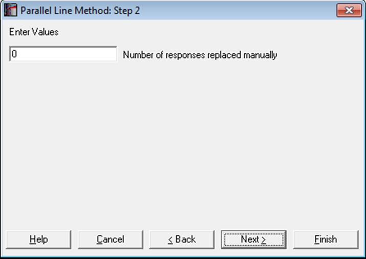
There is one small problem though; there is normally no such dialogue in bioassay procedures. By default, this input box is not displayed, because it is needed by a relatively small number users and it may create compliance problems during day-to-day use. To display the Number of responses replaced manually input box you need to enter the following line in:
C:\ProgramData\Unistat\Unistat10\Unistat10.ini
file under the [Bioassay] section:
ShowReplaceBox=1
We have already mentioned that in Quantal Response Method and Four-Parameter Logistic Model procedures replacement of outliers will probably never be needed, because simply deleting an outlier is superior to replacing it with an estimated value.
Example
Let us go back to the Latin Square example given in section 10.0.6.4. Automatic Outlier Replacement, where the first run on data not only marked case 3 as a possible outlier, but also gave us an Estimated Response value of 175.4444. We can now replace the outlier value of 162 with this estimated value in the spreadsheet and run the Latin Square procedure again. This time we must ensure that the Number of responses replaced manually input box was made available and enter 1 in the box.

Parallel Line Method
Latin Square Design
Validity of Assay
|
Due To |
Sum of Squares |
DoF |
Mean Square |
F-Stat |
Prob |
|
Preparations |
1.194 |
1 |
1.194 |
0.065 |
0.8018 |
|
Linear Regression |
8475.042 |
1 |
8475.042 |
460.157 |
0.0000 |
|
Non-parallelism |
18.375 |
1 |
18.375 |
0.998 |
0.3304 |
|
Non-linearity |
4.642 |
2 |
2.321 |
0.126 |
0.8823 |
|
Quadratic Regression |
1.963 |
1 |
1.963 |
0.107 |
0.7476 |
|
Quadratic Difference |
2.679 |
1 |
2.679 |
0.145 |
0.7071 |
|
Treatments |
8499.253 |
5 |
1699.851 |
|
|
|
Blocks(Rows) |
347.475 |
5 |
69.495 |
3.773 |
0.0153 |
|
Blocks(Columns) |
158.623 |
5 |
31.725 |
1.723 |
0.1778 |
|
Residual |
349.937 |
19 |
18.418 |
|
|
|
Total |
9355.288 |
34 |
275.156 |
|
|
1 responses have been replaced.
Case (Diagnostic) Statistics
|
|
Response |
Dose |
Preparations |
Rows |
Columns |
Estimated Response |
Residuals |
Standardised Residuals |
|
1 |
161 |
1 |
Standard S |
1 |
1 |
157.7639 |
3.2361 |
0.6174 |
|
2 |
151 |
1 |
Preparation T |
2 |
1 |
157.3997 |
-6.3997 |
-1.2210 |
|
3 |
175.4444 |
1.5 |
Preparation T |
3 |
1 |
176.1914 |
-0.7470 |
-0.1425 |
|
4 |
194 |
2.25 |
Standard S |
4 |
1 |
195.3472 |
-1.3472 |
-0.2570 |
|
5 |
176 |
1.5 |
Standard S |
5 |
1 |
176.5556 |
-0.5556 |
-0.1060 |
|
6 |
193 |
2.25 |
Preparation T |
6 |
1 |
194.9830 |
-1.9830 |
-0.3784 |
|
7 |
160 |
1 |
Preparation T |
1 |
2 |
157.3997 |
2.6003 |
0.4961 |
|
8 |
192 |
2.25 |
Preparation T |
2 |
2 |
194.9830 |
-2.9830 |
-0.5691 |
|
9 |
195 |
2.25 |
Standard S |
3 |
2 |
195.3472 |
-0.3472 |
-0.0662 |
|
10 |
184 |
1.5 |
Standard S |
4 |
2 |
176.5556 |
7.4444 |
1.4204 |
|
… |
… |
… |
… |
… |
… |
… |
… |
… |
Potency
Latin Square Design
|
|
Estimated Potency |
Lower 95% |
Upper 95% |
DoF |
|
Preparation T |
0.9922 |
0.9297 |
1.0586 |
19 |
1 responses have been replaced.
10.0.7. Prediction, Interpolation, Extrapolation
Example
Open BIOPHARMA9 and locate columns C27, C28 and L29. Add three lines to the data in rows 25, 26 and 27 as follows.
|
|
Response |
Dose |
Preparations |
|
1 |
18 |
1 |
Standard S |
|
2 |
22.8 |
2 |
Standard S |
|
3 |
30.4 |
3 |
Standard S |
|
… |
… |
… |
… |
|
23 |
23.1 |
3 |
Preparation U |
|
24 |
27 |
4 |
Preparation U |
|
25 |
* |
4 |
Standard S |
|
26 |
16.8 |
* |
Preparation T |
|
27 |
* |
2 |
Preparation U |
Select Bioassay → Parallel Line Method. From the Variable Selection Dialogue select the first option Completely Randomised Design and then select columns C27, C28 and L29 respectively as [Data], [Dose], and [Preparation] Click [Next] to proceed to Output Options Dialogue and click on the [Opt] button situated to the left of Case (Diagnostic) Statistics option. Check only the Response, Dose, Preparations and Estimated Response options and click [Finish].
Parallel Line Method
3 row(s) omitted due to missing values
Completely Randomised Design
Case (Diagnostic) Statistics
|
|
Response |
Dose |
Preparations |
Estimated Response |
|
1 |
18 |
1 |
Standard S |
17.8264 |
|
2 |
22.8 |
2 |
Standard S |
25.8732 |
|
3 |
30.4 |
3 |
Standard S |
30.5803 |
|
… |
… |
… |
… |
… |
|
23 |
23.1 |
3 |
Preparation U |
24.9803 |
|
24 |
27 |
4 |
Preparation U |
28.3200 |
|
* 25 |
* |
4 |
Standard S |
33.9200 |
|
& 26 |
16.8 |
1.005275124572 |
Preparation T |
* |
|
* 27 |
* |
2 |
Preparation U |
20.2732 |
Estimated responses marked by ‘*’ are predicted.
Doses marked by ‘&’ are predicted.
