8.5. Factor Analysis
While the aim of Principal Components Analysis is simply to transform the original variables into a new set of variables, Factor Analysis attempts to construct a mathematical model explaining the correlations between a large set of variables. The Factor Analysis does this by deriving some variables (factors) that cannot be observed directly from the raw data.
8.5.1. Factoring Methods
The Factor Analysis is based on the Principal Components Analysis (see Mardia, K. V., Kent, J. T. and Bibby, J. M., 1979). UNISTAT provides two variations of this method called Principal Components Factoring and Principal Axis Factoring. Central to both methods is the concept of communality, which is the squared multiple correlations for each factor with all other factors and represent the proportion of variance explained by the common factors. When the number of factors is set to its maximum (the number of variables), communalities become unity and the Factor Analysis is reduced to a Principal Components Analysis.
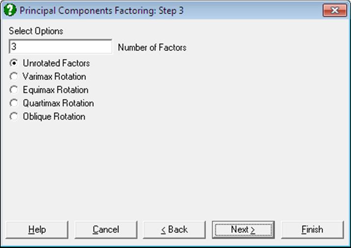
Principal Components Factoring: This procedure will first perform a Principal Components Analysis and determine the number of components with an eigenvalue greater than unity. This number will be displayed in a dialogue as the number of factors to be extracted, and it can be changed to any value between one and the total number of variables. Then you can either display the unrotated factors or proceed with one of the four rotation options available.
Principal Axis Factoring: First a Principal Components Analysis is performed and the communalities are computed for the selected number of factors. At this stage, it is possible to display the eigenvalues and eigenvectors or to proceed with the next stage of the analysis.
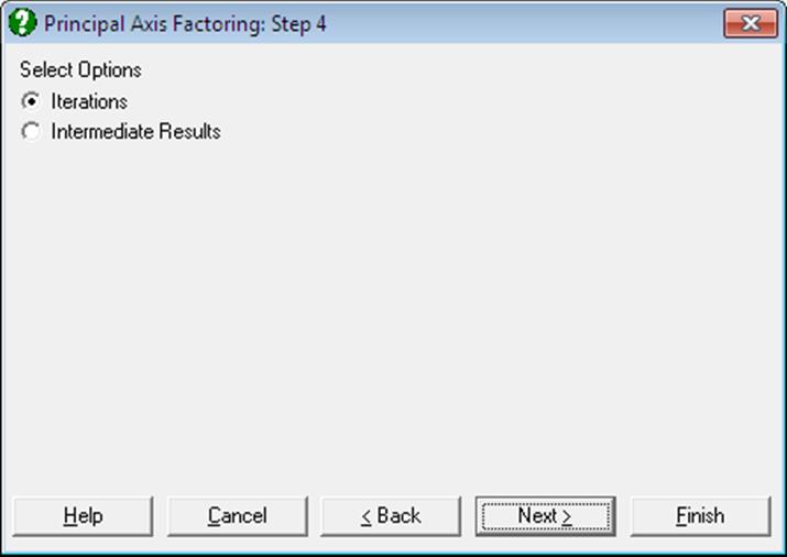
These initial communalities are then substituted into the diagonal of the correlation matrix replacing ones, and then another PCA is performed and the new communalities are computed. Iterations continue until the maximum number of iterations is reached or the change in the communality estimates is less than the given tolerance level.
8.5.2. Unrotated Output Options
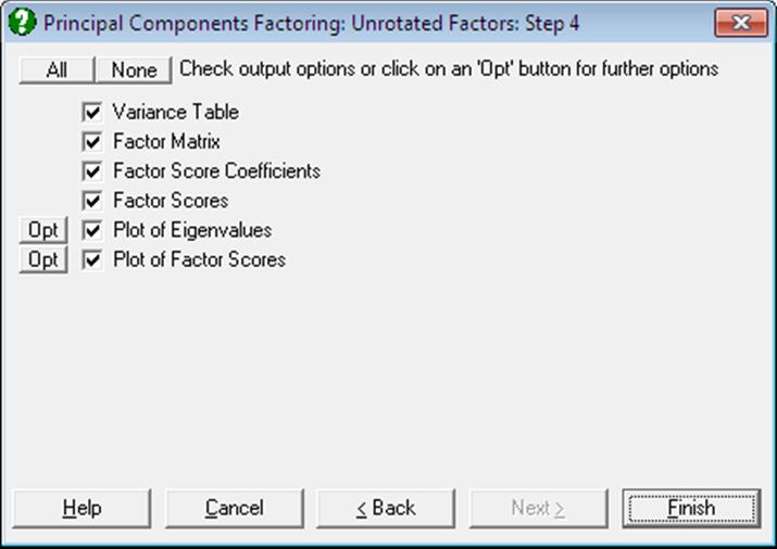
The Principal Components Factoring and Principal Axis Factoring methods offer the same initial results menu, also providing access to various rotation options.
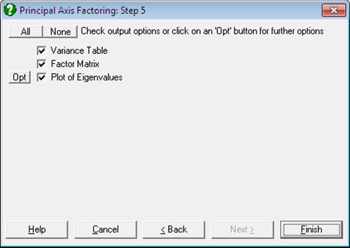
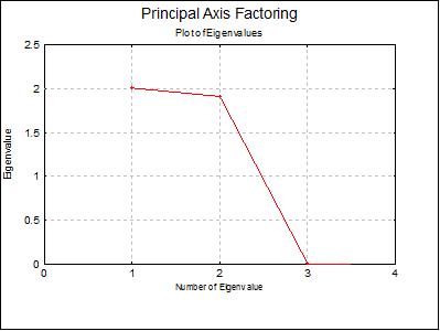
Variance Table: This table is similar to the table of eigenvalues discussed in Principal Components Analysis (also see plot of eigenvalues or scree plot), except that only the selected number of factors are displayed and there is a new column called communalities – the squared multiple correlations for each selected factor with all other factors.
As we have seen above, the program will select by default only those factors with an eigenvalue greater than unity. By examining this table, however, you may wish to adopt a different criterion and choose, say, the first r factors which explain 90% of the variation in data. In this case, press <Escape/Back> twice to edit the number of factors suggested by the program, and display the Variance Table again. This process does not involve recomputing the principal components.
Factor Matrix: Elements of this matrix are commonly referred to as factor loadings since they indicate how much weight is assigned to each factor. Factor loadings are the correlations between the derived factors and the original variables and are used to establish the link between the two sets. The factors can then be interpreted as representing those characteristics of the original data with which they have the highest correlations. For instance, if the principal component number 1’s correlation with the original variable called intelligence is the highest, it may then be said to represent intelligence. Of course, other original variables will also be correlated with the first principal component, representing other influences on intelligence.
Factor Score Coefficients: When multiplied by the original data matrix, these coefficients will transform the original data to a smaller set representing the values of factors. This is the matrix of unrotated factor score coefficients. After a rotation is performed, the rotated factor score coefficients will also be given. These coefficients may be saved to the Data Processor to transform various related data sets outside the procedure. If the data input is a raw data matrix, then the transformation will be carried out by the procedure and the results will be displayed in tabular and graphical forms.
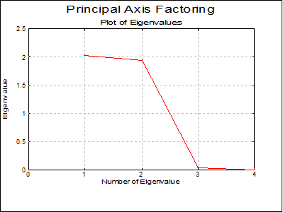
Plot of Eigenvalues (Scree Plot): This is also called the scree plot. Eigenvalues are sorted in decreasing order. Typically, this plot will fall sharply with the first few eigenvalues and then get less and less steep.
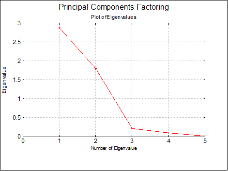
You can edit properties of the graph by selecting Edit → XY Points from the menu.
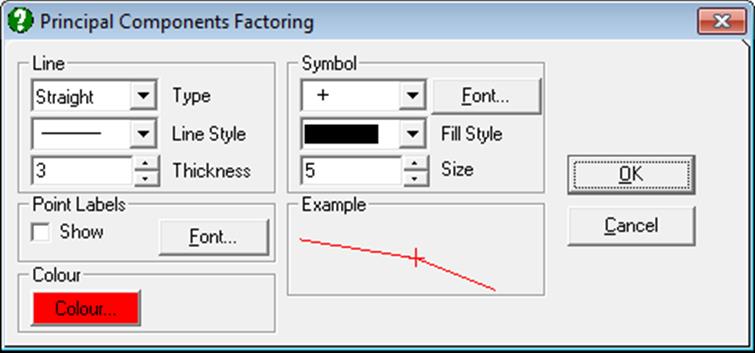
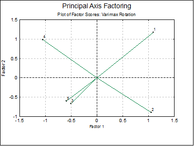
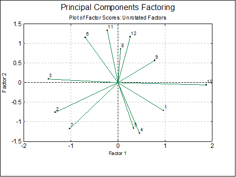
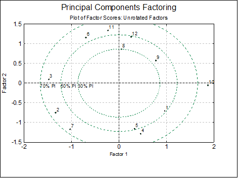
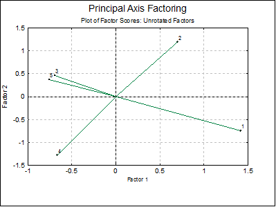
Table and Plot of Factor Scores: These are the derived variables representing most of the variation in the original data, and as such are analogous to principal components in the Principal Components Analysis. Factor scores may be saved for further analysis.
When the input data for the analysis is a correlation or covariance matrix, the table and plot of factor scores options will not be available.
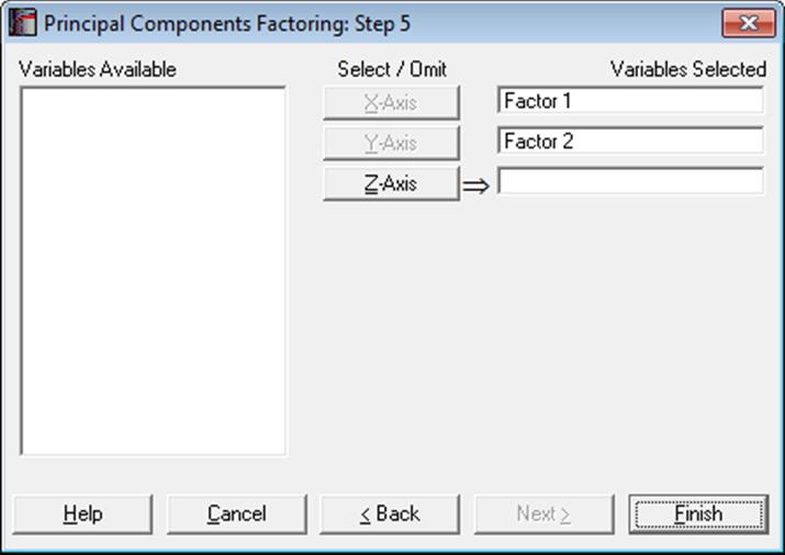
The program will display a 2D graph if you select two variables to plot, and a 3D graph if you select three variables.
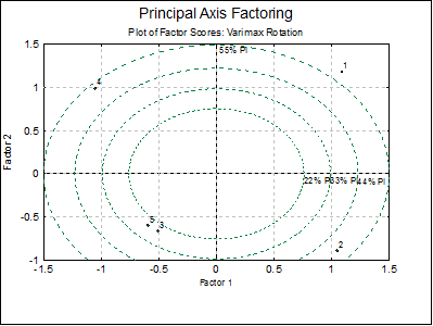
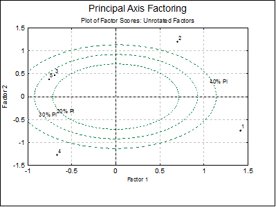
You can edit properties of the graph by selecting Edit → XY Points from the menu. If you select the Ellipse option from the Line Type list, a further dialogue will pop up allowing you to draw interval ellipses for the mean of Y (confidence) and / or actual Y (prediction) values at one or more confidence levels.
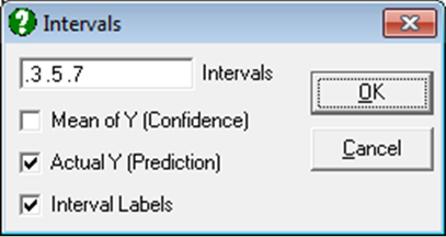
Either or both intervals or none can be drawn by checking the boxes as desired. The text box can be used to enter multiple confidence levels between 0 and 1, separated by spaces. When the last box is checked, a label will be printed for each interval curve. For further details see Ellipse For further details see Ellipse Confidence and Prediction Intervals in 4.1.1.1.1. Line.
8.5.3. Rotations

Often, the first phase of the analysis will produce factor loadings showing correlations between all factors and all original variables, making it difficult to assign meaningful attributes to factors. It is possible to improve interpretation of factors by rotating the factor matrix.
There are two major types of rotation; orthogonal, keeping the axes at right angles, and oblique, where angles between axes are not necessarily 90º. UNISTAT supports three orthogonal (varimax, equimax and quartimax) and one oblique (oblimin) rotation. All these are iterational procedures and may take a long time to compute. The oblimin method also requires the input of a parameter (Delta) which determines the degree of obliqueness.
The outputs for orthogonal and oblique rotations are also slightly different. However, all rotation options will display the rotated factor matrix, plot of factors and factor score coefficients. If the input data is not a correlation or covariance matrix, then the factor scores will also be displayed in tabular and graphical forms.
Orthogonal Rotations: The most popular rotation method is varimax, which minimises the number of variables that have high loadings. Quartimax method, on the other hand, minimises the number of factors needed to explain a variable. Equimax is a combination of varimax and quartimax methods.
The orthogonal rotation output options include the final communalities and the factor transition matrix. The latter is the matrix which affects rotations when multiplied by the original factors.
Oblimin Rotation: A parameter determining the degree of obliqueness (Delta) is entered by the user. This usually varies from 0 to negative numbers, 0 giving the most oblique solution. Oblimin is an iterational method involving highly demanding calculations, including determining the roots of a third degree polynomial at each iteration.
In addition to the output options of the orthogonal rotation, the structure matrix and the factor correlations matrix options are also available for oblimin rotation.
8.5.4. Rotated Output Options
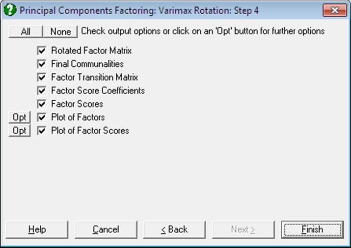
Rotated factors, factor score coefficients and factor scores can be displayed in tabular or graphical form. The factor scores options will not be available when a correlation or covariance matrix is input.
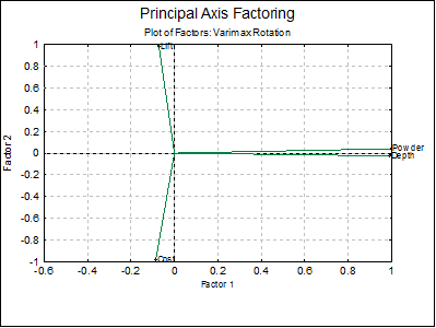
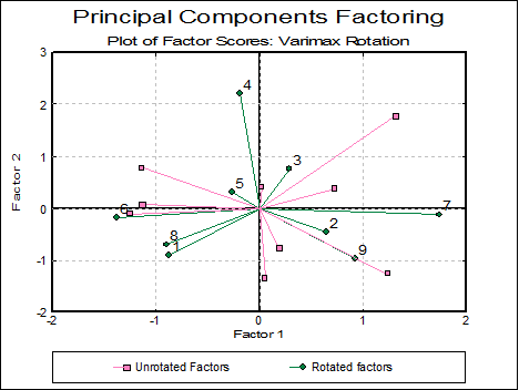
The plot of factors option allows display of both unrotated and rotated factors on the same graph, enabling you to compare the effects of rotation. The rotated factors can be greater than unity after an oblique rotation. The factor scores graph may take a long time to draw due to the amount of computing necessary, particularly when the number of factors is relatively large.
8.5.5. Factor Analysis Example
Table 12.2 on p. 607 from Tabachnick, B. G. & L. S. Fidell (1989).
Open MULTIVAR, select Statistics 2 → Factor Analysis → Principal Axis Factoring and select Cost, Lift, Depth and Powder (C6 to C9) as [Variable]s. The output contains three stages. First, initial communalities, eigenvalues and factor matrix are reported. Then, the final communalities and eigenvalues and thirdly, the results after Varimax rotation.
Principal Axis Factoring
Variance Table
|
|
Communality |
Factor |
Eigenvalue |
Percent |
Cumulative |
|
Cost |
0.9608 |
1 |
2.0163 |
50.4% |
50.4% |
|
Lift |
0.9532 |
2 |
1.9415 |
48.5% |
98.9% |
|
Depth |
0.9900 |
|
|
|
|
|
Powder |
0.9909 |
|
|
|
|
Factor Matrix
|
|
Factor 1 |
Factor 2 |
|
Cost |
-0.5004 |
0.8560 |
|
Lift |
0.3566 |
-0.9249 |
|
Depth |
0.8909 |
0.4490 |
|
Powder |
0.9193 |
0.3896 |
Principal Axis Factoring: Unrotated Factors
Variance Table
|
|
Communality |
Factor |
Eigenvalue |
Percent |
Cumulative |
|
Cost |
0.9719 |
1 |
2.0052 |
50.1% |
50.1% |
|
Lift |
0.9587 |
2 |
1.9101 |
47.8% |
97.9% |
|
Depth |
0.9852 |
|
|
|
|
|
Powder |
0.9995 |
|
|
|
|
Factor Matrix
|
|
Factor 1 |
Factor 2 |
|
Cost |
-0.4049 |
0.8989 |
|
Lift |
0.2548 |
-0.9454 |
|
Depth |
0.9283 |
0.3515 |
|
Powder |
0.9564 |
0.2913 |
Factor Score Coefficients
|
|
Factor 1 |
Factor 2 |
|
Cost |
0.0121 |
0.6664 |
|
Lift |
0.2914 |
-0.3046 |
|
Depth |
-0.1813 |
-0.1372 |
|
Powder |
1.1480 |
0.5027 |
Factor Scores
|
|
Factor 1 |
Factor 2 |
|
1 |
1.4177 |
-0.7455 |
|
2 |
0.6990 |
1.1896 |
|
3 |
-0.6946 |
0.4601 |
|
4 |
-0.6661 |
-1.2735 |
|
5 |
-0.7560 |
0.3693 |
Principal Axis Factoring: Varimax rotation
Rotated Factor Matrix
|
|
Factor 1 |
Factor 2 |
|
Cost |
-0.0860 |
-0.9821 |
|
Lift |
-0.0710 |
0.9765 |
|
Depth |
0.9922 |
-0.0259 |
|
Powder |
0.9990 |
0.0403 |
Final Communalities
|
|
Communality |
|
Cost |
0.9719 |
|
Lift |
0.9587 |
|
Depth |
0.9852 |
|
Powder |
0.9995 |
Factor Transition Matrix
|
|
Factor 1 |
Factor 2 |
|
Factor 1 |
0.9441 |
-0.3296 |
|
Factor 2 |
0.3296 |
0.9441 |
Factor Score Coefficients
|
|
Factor 1 |
Factor 2 |
|
Cost |
0.2310 |
-0.6252 |
|
Lift |
0.1747 |
0.3837 |
|
Depth |
-0.2164 |
0.0698 |
|
Powder |
1.2496 |
-0.0963 |
Factor Scores
|
|
Factor 1 |
Factor 2 |
|
1 |
1.0928 |
1.1712 |
|
2 |
1.0521 |
-0.8927 |
|
3 |
-0.5042 |
-0.6634 |
|
4 |
-1.0486 |
0.9827 |
|
5 |
-0.5920 |
-0.5978 |
