10.6.1. Cylinder-Plate 5+1 Assay
This is an implementation of the cylinder-plate assay defined in United States Pharmacopoeia (2010) Chapter <81> Antibiotics-Microbial Assays, which is widely known as the 5+1 assay. Thanks to its flexible data entry method, UNISTAT can cater for many different types of data configuration. See examples 1 and 2 below.

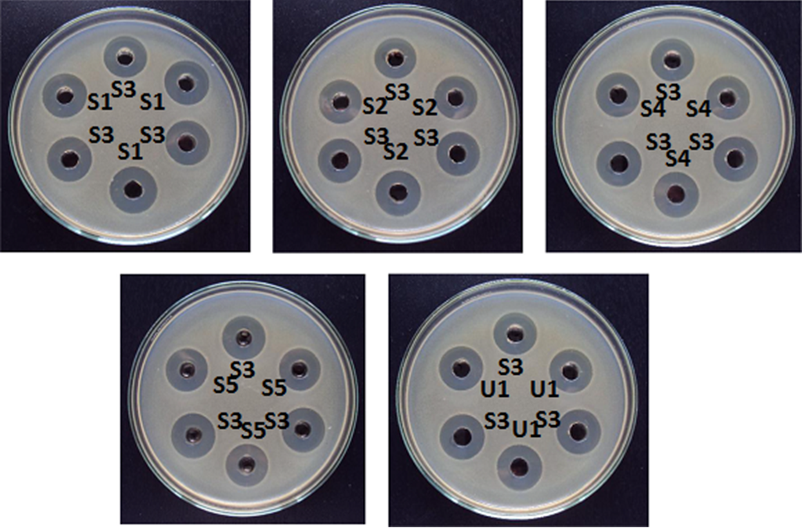
Assay design according to USP <81> consists of five concentrations of the standard preparation and one concentration each for one or more unknown preparations. The first four plates contain different concentrations of the standard preparation. One or more plates can be added for unknown (or test) preparations. Each plate contains six wells and only two treatments. Odd numbered wells on all plates contain the median standard concentration S3. Even numbered wells on the first four plates contain the remaining standard concentrations of S1, S2, S4 and S5. Even numbered wells on the fifth, sixth, etc. plates contain the unknown preparations U1, U2, etc.
This table shows the dose configuration of a 5+1 design with two test preparations, which constitutes one replicate.
|
Plates \ Wells |
1 |
2 |
3 |
4 |
5 |
6 |
|
1 |
S3 |
S1 |
S3 |
S1 |
S3 |
S1 |
|
2 |
S3 |
S2 |
S3 |
S2 |
S3 |
S2 |
|
3 |
S3 |
S4 |
S3 |
S4 |
S3 |
S3 |
|
4 |
S3 |
S5 |
S3 |
S5 |
S3 |
S4 |
|
5 |
S3 |
U1 |
S3 |
U1 |
S3 |
U1 |
|
6 |
S3 |
U2 |
S3 |
U2 |
S3 |
U2 |
|
… |
… |
… |
… |
… |
… |
… |
In each replicate with one unknown (i.e. a set of five plates) there are 15 median standard concentrations S3, three of each one of other four standard concentrations S1, S2, S4, S5 and three of the unknown U1. There are usually three replicates, totalling 15 plates and 90 wells.
This data is entered into a spreadsheet for analysis with UNISTAT as in the following table, where Rows and Columns variables refer to the rows (Plates) and columns (Wells) of the above table. The Response and Dose variables are numeric and Rows and Columns are alphanumeric. Ordering of the plates and replicates is not significant, as long as the rows of the table are kept intact. The odd column numbers should always correspond to the median standard concentration of S3. The Replicates column here is for reference only and is not required as a variable in the analysis.
|
Response |
Dose |
Rows |
Columns |
Replicates |
|
D1 |
S3 |
1 |
1 |
1 |
|
D2 |
S1 |
1 |
2 |
1 |
|
D3 |
S3 |
1 |
3 |
1 |
|
D4 |
S1 |
1 |
4 |
1 |
|
D5 |
S3 |
1 |
5 |
1 |
|
D6 |
S1 |
1 |
6 |
1 |
|
D7 |
S3 |
2 |
1 |
1 |
|
D8 |
S2 |
2 |
2 |
1 |
|
D9 |
S3 |
2 |
3 |
1 |
|
D10 |
S2 |
2 |
4 |
1 |
|
D11 |
S3 |
2 |
5 |
1 |
|
D12 |
S2 |
2 |
6 |
1 |
|
D13 |
S3 |
3 |
1 |
1 |
|
D14 |
S4 |
3 |
2 |
1 |
|
D15 |
S3 |
3 |
3 |
1 |
|
D16 |
S4 |
3 |
4 |
1 |
|
D17 |
S3 |
3 |
5 |
1 |
|
D18 |
S4 |
3 |
6 |
1 |
|
D19 |
S3 |
4 |
1 |
1 |
|
D20 |
S5 |
4 |
2 |
1 |
|
D21 |
S3 |
4 |
3 |
1 |
|
D22 |
S5 |
4 |
4 |
1 |
|
D23 |
S3 |
4 |
5 |
1 |
|
D24 |
S5 |
4 |
6 |
1 |
|
D25 |
S3 |
5 |
1 |
1 |
|
D26 |
U1 |
5 |
2 |
1 |
|
D27 |
S3 |
5 |
3 |
1 |
|
D28 |
U1 |
5 |
4 |
1 |
|
D29 |
S3 |
5 |
5 |
1 |
|
D30 |
U1 |
5 |
6 |
1 |
|
D31 |
S3 |
1 |
1 |
2 |
|
D32 |
S1 |
1 |
2 |
2 |
|
D33 |
S3 |
1 |
3 |
2 |
|
D34 |
S1 |
1 |
4 |
2 |
|
D35 |
S3 |
1 |
5 |
2 |
|
D36 |
S1 |
1 |
6 |
2 |
|
D37 |
S3 |
2 |
1 |
2 |
|
… |
… |
… |
… |
… |
UNISTAT first calculates the corrected means and related statistics as described in Table 13 of US Pharmacopoeia (2010) Chapter <81> and displays this information in the output. The corrected means are then analysed using the Parallel Line Method. Because 5+1 assays will always have a zero residual degree of freedom, fiducial confidence limits of the estimated potency is based on the linearity sum of squares and degrees of freedom. Note that USP does not report confidence limits of the estimated potency.
It is also possible to run multiple 5+1 assays and to combine their results in a single run. See section 10.0.4. Multiple Assays with Combination.
Example 1
Data is given in Table 13 of US Pharmacopoeia (2010) Chapter <81>.
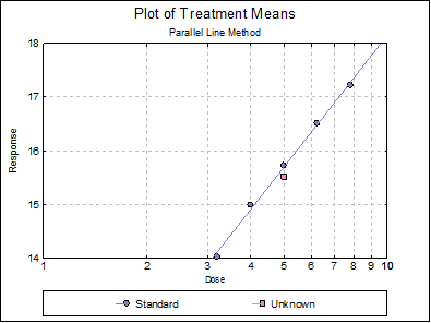
Open SPECIFICASSAYS and select Bioassay → Specific Assays → Cylinder-Plate 5+1 Assay. From the Variable Selection Dialogue select C2 Response, C3 Dose, C4 Rows, C5 Columns, as [Response], [Dose], [Row Factor] and [Col Factor] respectively. From the Output Options Dialogue check the Data, Validity of Assay, Potency and Plot of Treatments options and click [Finish] to obtain the following output.
Parallel Line Method
Completely Randomised Design
5+1 Assay
|
Preparations |
Dose |
Mean (Odd well nos) |
Standard Deviation |
%RSD |
|
Standard |
3.2 |
15.8667 |
0.2000 |
1.3 |
|
Standard |
4 |
15.5667 |
0.1581 |
1.0 |
|
Standard |
5 |
15.7222 |
|
|
|
Standard |
6.25 |
15.7889 |
0.1691 |
1.1 |
|
Standard |
7.8125 |
15.6667 |
0.1414 |
0.9 |
|
Sample 1 |
5 |
15.6778 |
0.1787 |
1.1 |
|
Preparations |
Mean (Even well nos) |
Standard Deviation |
%RSD |
Corrected Means |
|
Standard |
14.1667 |
0.3240 |
2.3 |
14.0222 |
|
Standard |
14.8333 |
0.2646 |
1.8 |
14.9889 |
|
Standard |
|
|
|
15.7222 |
|
Standard |
16.5778 |
0.2333 |
1.4 |
16.5111 |
|
Standard |
17.1667 |
0.2236 |
1.3 |
17.2222 |
|
Sample 1 |
15.4778 |
0.3073 |
2.0 |
15.5222 |
Data
|
|
Response |
Dose |
Preparations |
|
1 |
14.02222222222 |
3.2 |
Standard |
|
2 |
14.98888888889 |
4 |
Standard |
|
3 |
15.72222222222 |
5 |
Standard |
|
4 |
16.51111111111 |
6.25 |
Standard |
|
5 |
17.22222222222 |
7.8125 |
Standard |
|
6 |
15.52222222222 |
5 |
Sample 1 |
Validity of Assay
|
Due To |
Sum of Squares |
DoF |
Mean Square |
F-Stat |
Prob |
|
Preparations |
0.024 |
1 |
0.024 |
3.699 |
0.1502 |
|
Linear Regression |
6.276 |
1 |
6.276 |
951.408 |
0.0001 |
|
Non-linearity |
0.020 |
3 |
0.007 |
|
|
|
Standard Non-linearity |
0.020 |
3 |
0.007 |
|
|
|
Sample 1 Non-linearity |
0.000 |
0 |
|
|
|
|
Treatments |
6.320 |
5 |
1.264 |
|
|
|
Residual |
0.000 |
0 |
|
|
|
|
Total |
6.320 |
5 |
1.264 |
|
|
Potency
0 residual SSQ and DoF replaced by non-linearity SSQ and DoF.
|
|
Estimated Potency |
Lower 95% |
Upper 95% |
DoF |
|
Sample 1 |
0.9529 |
0.8789 |
1.0321 |
3 |
|
|
Relative Potency |
Lower 95% |
Upper 95% |
|
Sample 1 |
95.29% |
87.89% |
103.21% |
|
|
Percent CI |
Lower 95% |
Upper 95% |
|
Sample 1 |
100.00% |
92.23% |
108.31% |

Example 2
Consider the following fictitious data set consisting of five doses of standard and one of unknown. There are 9 replicates.
|
|
S1 |
S3 |
S2 |
S3 |
S4 |
S3 |
S5 |
S3 |
U |
S3 |
|
1 |
19.04 |
19.22 |
19.69 |
20.22 |
20.04 |
19.21 |
20.57 |
19.66 |
18.34 |
18.01 |
|
2 |
17.15 |
19.16 |
18.23 |
17.18 |
19.08 |
19.53 |
20.54 |
17.21 |
19.33 |
18.36 |
|
3 |
17.42 |
18.87 |
18.33 |
18.95 |
19.81 |
19.96 |
20.88 |
18.97 |
19.04 |
19.04 |
|
4 |
14.11 |
19.34 |
19.57 |
19.2 |
20.39 |
19.44 |
20.69 |
18.93 |
19.07 |
19.44 |
|
5 |
17.45 |
18.25 |
19.29 |
17.74 |
19.99 |
20.19 |
20.38 |
19.81 |
18.66 |
19.14 |
|
6 |
17.85 |
19.37 |
17.95 |
19.28 |
19.58 |
18.19 |
20.11 |
18.71 |
19.42 |
19.4 |
|
7 |
18.85 |
20.03 |
19.1 |
20.36 |
19.87 |
19.65 |
20.04 |
20.03 |
19.01 |
19.02 |
|
8 |
17.67 |
18.04 |
17.78 |
18.8 |
20 |
18.77 |
20.91 |
19.17 |
18.93 |
19.2 |
|
9 |
18.65 |
19.64 |
20.26 |
19.5 |
20.04 |
19.83 |
20.61 |
19.46 |
18.84 |
18.73 |
where:
|
|
Dose |
|
S1 |
25.6 |
|
S2 |
32 |
|
S3 |
40 |
|
S4 |
50 |
|
S5 |
62.5 |
|
U |
40 |
Irrespective of their actual locations on the plates this data can be entered into UNISTAT as in the example file SPECIFICASSAYS columns C7 to C11. Note that the odd numbered columns contain S3 and even numbered columns other doses. Values of the Rows variable correspond to distinct dose levels. Also, to take 10-based logarithm of dose values (instead of natural logarithm, which is the default) you can enter the following line:
LogBase10=1
C:\ProgramData\Unistat\Unistat10\Unistat10.ini
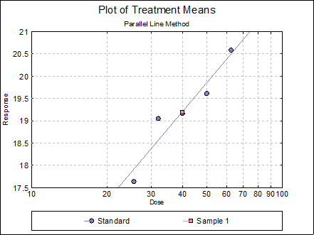
Open SPECIFICASSAYS and select Bioassay → Specific Assays → Cylinder-Plate 5+1 Assay. From the Variable Selection Dialogue select C8 Response, C9 Dose, C10 Rows, C11 Columns, as [Response], [Dose], [Row Factor] and [Col Factor] respectively. From the Output Options Dialogue check the Data, Validity of Assay, Potency and Plot of Treatments options and click [Finish] to obtain the following output.
Parallel Line Method
Completely Randomised Design
5+1 Assay
|
Preparations |
Dose |
Mean (Odd well nos) |
Standard Deviation |
%RSD |
|
Standard |
25.6 |
19.1022 |
0.6328 |
3.3 |
|
Standard |
32 |
19.0256 |
1.0394 |
5.5 |
|
Standard |
40 |
19.1631 |
|
|
|
Standard |
50 |
19.4189 |
0.6222 |
3.2 |
|
Standard |
62.5 |
19.1056 |
0.8357 |
4.4 |
|
Sample 1 |
40 |
18.9267 |
0.4782 |
2.5 |
|
Preparations |
Mean (Even well nos) |
Standard Deviation |
%RSD |
Corrected Means |
|
Standard |
17.5767 |
1.4679 |
8.4 |
17.6375 |
|
Standard |
18.9111 |
0.8692 |
4.6 |
19.0486 |
|
Standard |
|
|
|
19.1631 |
|
Standard |
19.8667 |
0.3659 |
1.8 |
19.6108 |
|
Standard |
20.5256 |
0.3040 |
1.5 |
20.5831 |
|
Sample 1 |
18.9600 |
0.3277 |
1.7 |
19.1964 |
Separate Regression
|
|
Intercept |
Slope |
Residual SS |
R-squared |
|
Standard |
8.5403 |
6.6591 |
0.3824 |
0.9159 |
|
Sample 1 |
* |
* |
* |
* |
Common Regression
|
|
Intercept |
Slope |
Residual SS |
R-squared |
|
Standard |
8.5403 |
6.6591 |
0.3824 |
0.9159 |
|
Sample 1 |
8.5281 |
|
|
|
|
Residual Variance = |
0.1275 |
|
Degrees of Freedom = |
3 |
Validity of Assay
|
Due To |
Sum of Squares |
DoF |
Mean Square |
F-Stat |
Prob |
|
Preparations |
0.000 |
1 |
0.000 |
0.001 |
0.9770 |
|
Linear Regression |
4.165 |
1 |
4.165 |
32.672 |
0.0106 |
|
Non-linearity |
0.382 |
3 |
0.127 |
|
|
|
Standard Non-linearity |
0.382 |
3 |
0.127 |
|
|
|
Sample 1 Non-linearity |
0.000 |
0 |
|
|
|
|
Treatments |
4.547 |
5 |
0.909 |
|
|
|
Residual |
0.000 |
0 |
|
|
|
|
Total |
4.547 |
5 |
0.909 |
|
|
Potency
0 residual SSQ and DoF replaced by non-linearity SSQ and DoF.
|
|
Estimated Potency |
Lower 95% |
Upper 95% |
DoF |
% Precision |
|
Sample 1 |
0.9958 |
0.5920 |
1.6686 |
3 |
59.45% |
|
|
Relative Potency |
Lower 95% |
Upper 95% |
|
Sample 1 |
99.58% |
59.20% |
166.86% |
|
|
Percent CI |
Lower 95% |
Upper 95% |
|
Sample 1 |
100.00% |
59.45% |
167.57% |
|
G = |
0.3100 |
|
C = |
1.4492 |

