9.3.5. Weibull Analysis
Two or three parameter Weibull models can be estimated employing maximum likelihood or ordinary least squares (OLS) regression methods. The program reports the estimated parameters, their confidence intervals and covariance matrix and features an interpolation facility.
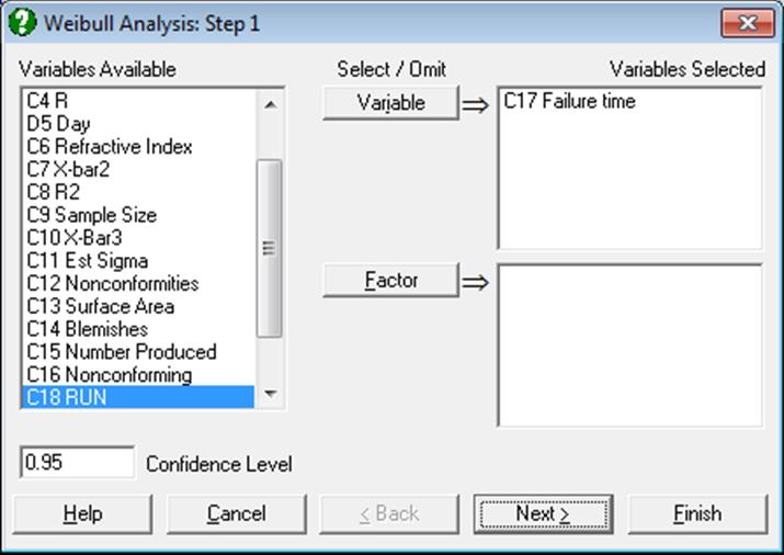
It is sufficient to select one data column to run a Weibull Analysis. Multisample data can be selected either in the form of multiple columns (not necessarily of equal length) or data columns classified by one or more factor columns (see 6.0.4. Multisample Tests). If at least one factor column is selected, then a further dialogue will pop up asking for the combination of factor levels to be included.
9.3.5.1. Weibull Inputs
An Intermediate Inputs dialogue enables you to control the following parameters:
Model: This can be one of two-parameter maximum likelihood or two- or three-parameter OLS regressions.
Method: If the method is OLS, then you can choose to regress Y on X (the default) or X on Y.
Population size: If the population size is known, you can enter it here. This is the number N used in generating the median ranks as described below. If this box is left as 0, then the program assumes that N is equal to the number of cases in the sample n.
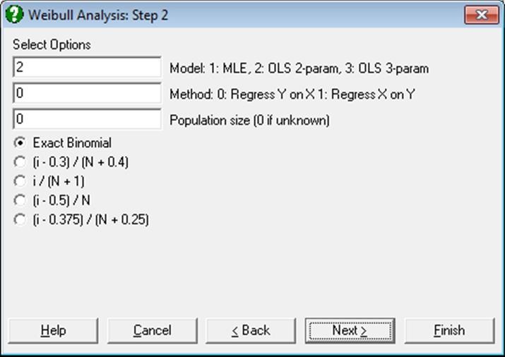
Median Ranks: In order to run a regression and to plot a chart, Weibull Analysis needs to generate median ranks as Y-axis values. Median ranks can be computed in one of the following ways.
· Exact Binomial
· (i – 0.3) / (N + 0.4)
· i / (N + 1)
· (i – 0.5) / N
· (i – 0.375) / (N + 0.25)
where N is the population size supplied by the user as described above. If N is not known, it is assumed to be equal to the sample size n. The default method adopted by UNISTAT is Exact Binomial, where the exact median ranks are determined from the binomial distribution as:
![]()
where Ri is the median rank of the ith observation. Other options in this list are various approximations to median ranks. For large values of N not all exact median ranks can be computed. When this is the case, the program cannot proceed with the analysis. However, you can still run your model by selecting one of the approximation formulas.
In Stand-Alone Mode, you can generate a data column containing median ranks using the Data Processor’s MdRk(N) function (see 3.4.2.5. Statistical Functions).
9.3.5.2. Weibull Output Options
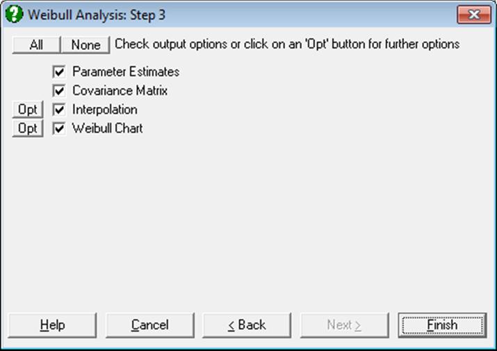
9.3.5.2.1. Weibull Parameter Estimates
Parameters of the Weibull distribution can be estimated by one of the following three methods.
Two-parameter maximum likelihood estimation: The probability density function for the two-parameter Weibull distribution is given as:
![]()
and the log likelihood function is:
![]()
where n is the sample size. Differentiating L with respect to β and η and setting equal to zero, we obtain the following two equations used in estimation:
![]()
![]()
Two-parameter OLS estimation: The cumulative distribution function for the two-parameter Weibull distribution is given as:
![]()
where T is the failure time, β is the shape parameter, η is the scale parameter. Taking the natural logarithm of both sides and rearranging we obtain:
![]()
This is clearly a line equation of the form:
![]()
where, conveniently, the left hand side is the gompit (or cloglog) function:
![]()
and F(T) is the median rank function, with the slope:
![]()
and the intercept:
![]()
Three-parameter OLS estimation: The cumulative distribution function for the three-parameter Weibull distribution is given as:

where β is the shape parameter, η is the scale parameter, and γ is the location parameter. This equation is linearised as above and all three parameters are estimated simultaneously using the iterative least squares method.
Mean failure time: This is found using the gamma function:
![]()
9.3.5.2.2. Weibull Covariance Matrix
For all estimation methods, the variance-covariance matrix is defined as the inverse of the second partial derivatives matrix of the log likelihood function:
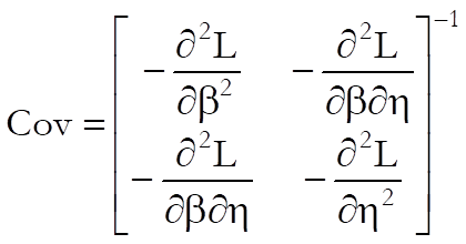
9.3.5.2.3. Weibull Interpolation
In the Output Options Dialogue, clicking on the [Opt] button situated to the left of the Interpolation check box, the interpolation dialogue can be accessed.
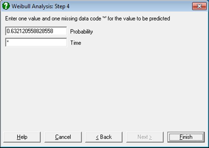
You can enter a failure probability to estimate the failure time or enter a failure time to estimate the probability of failure. Each time you will need to enter an asterisk for the parameter to be estimated. The program will display the estimated parameter together with its confidence interval.
9.3.5.2.4. Weibull Chart
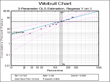
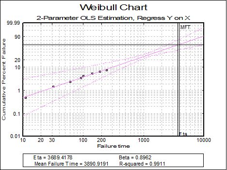
If you use UNISTAT’s X-Y Plots procedure and set the Y-axis scale as gompit and the X-axis scale as logarithmic, you instantly have a Weibull probability paper. If you select median ranks as the Y-axis and failure times as the X-axis variable and fit a trend line, you would have already estimated the two-parameter Weibull model. This is precisely the way we generate the Weibull chart here.
In Stand-Alone Mode, you can generate a data column containing median ranks using the Data Processor’s MdRk(N) function (see 3.4.2.5. Statistical Functions).
If the data lies on a near-straight line, then it is said to conform to the Weibull distribution.
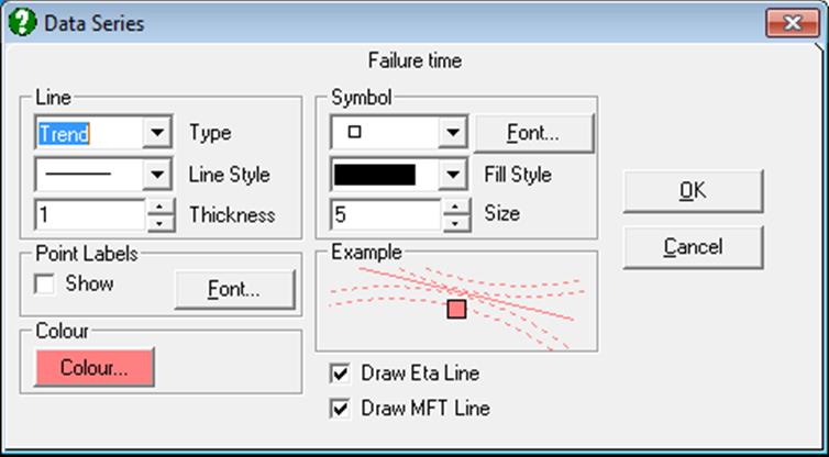
Clicking the [Opt] button situated to the left of the Weibull Chart option will place the graph in UNISTAT’s Graphics Editor. In the Edit → Data Series dialogue, two check boxes allow you to show or hide the eta and mean failure time lines on the chart.
9.3.5.3. Examples
Example 1
Example 16.15 on p. 580 from Banks, Jerry (1989). Failure times of 8 components are given. The population size is known to be 100.
Open TIMESER and select Statistics 2 → Quality Control → Weibull Analysis. From the Variable Selection Dialogue select Failure time (C17) as [Variable]. In the next dialogue, enter 100 for the population size and select (i – 0.5) / N for median rank approximation. The following output is obtained:
Weibull Analysis
Parameter Estimates
Data variable: Failure time
Number of Cases: 8
Population Size: 100
Median Rank Method: (i – 0.5) / N
2-Parameter OLS Estimation
Regress Y on X
|
|
Value |
Lower 95% |
Upper 95% |
|
Beta |
0.8962 |
0.5791 |
1.3870 |
|
Eta |
3689.4178 |
2098.0830 |
6487.7337 |
|
Mean Failure Time |
3890.9191 |
|
|
|
Correlation Coefficient = |
0.9956 |
|
R-squared = |
0.9911 |
Covariance Matrix
|
|
Beta |
Eta |
|
Beta |
0.0399 |
-192.7873 |
|
Eta |
-192.7873 |
1128917.0915 |
Interpolation
|
Probability |
Time |
Lower 95% |
Upper 95% |
|
0.632120558828558 |
3689.4178 |
2098.0830 |
6487.7337 |
Example 2
Continuing from the last example, this time select 3-parameter model with population size 0 (unknown) and Exact Binomial median ranks:
Weibull Analysis
Parameter Estimates
Data variable: Failure time
Number of Cases: 8
Median Rank Method: Exact Binomial
3-Parameter OLS Estimation
Regress Y on X
|
|
Value |
Lower 95% |
Upper 95% |
|
Beta |
1.4466 |
0.8149 |
2.5682 |
|
Eta |
143.7028 |
85.1939 |
242.3940 |
|
Gamma |
-15.9995 |
|
|
|
Mean Failure Time |
130.3404 |
|
|
|
Correlation Coefficient = |
0.9976 |
|
R-squared = |
0.9952 |
Covariance Matrix
|
|
Beta |
Eta |
|
Beta |
0.1795 |
1.7235 |
|
Eta |
1.7235 |
1469.3800 |
Interpolation
|
Probability |
Time |
Lower 95% |
Upper 95% |
|
0.632120558828558 |
143.7028 |
85.1939 |
242.3940 |
