3.3. Data Menu

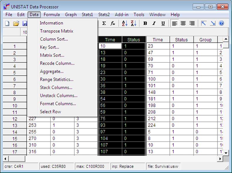
Various utilities are provided for transforming and formatting data. It is also possible to sort, key sort and recode data matrix columns or perform operations like Range Statistics and Aggregate.

Some of the options will not be active (i.e. they will be greyed out) unless a range of columns has been highlighted first.

3.3.1. Information

This procedure displays a basic statistics table for all data columns in Data Processor. The statistics displayed are the current values of Scalar Functions for each column. These are Len() (total number of observations including missing observations), Mis() (number of missing observations), Avg() (arithmetic mean), Std() (sample standard deviation), Var() (sample variance), Sum(), Ssq() (sum of squares), Min() (minimum observation), Max() (maximum observation) and the formulas, if any. In case a column contains missing values, the values of Avg(), Var() and Std() are adjusted for the number of missing observations.

If a Select Row variable is in effect, the number of rows omitted will also be reported and all statistics will be adjusted for the valid number of cases.

Example

Information

file: Anova.usw

	LEN	MIS	AVG	STD	VAR
C1 Hardness	16	0	1.2500	2.9326	8.6000
C2 Tip	16	0	2.5000	1.1547	1.3333
C3 Coupon	16	0	2.5000	1.1547	1.3333
C4 Operator	25	0	3.0000	1.4434	2.0833
C5 Batch	25	0	3.0000	1.4434	2.0833
C6 Formulation	25	0	String	String	String
C7 Coded Data	25	0	0.4000	5.3072	28.1667
C8 Test assemblies	25	0	String	String	String

 

	SUM	SSQ	MIN	MAX
C1 Hardness	20.0000	154.0000	-3.0000	7.0000
C2 Tip	40.0000	120.0000	1.0000	4.0000
C3 Coupon	40.0000	120.0000	1.0000	4.0000
C4 Operator	75.0000	275.0000	1.0000	5.0000
C5 Batch	75.0000	275.0000	1.0000	5.0000
C6 Formulation	String	String	A	E
C7 Coded Data	10.0000	680.0000	-8.0000	13.0000
C8 Test assemblies	String	String	a	e

 

Information on string, date and time variables will also be displayed under this option, though many of the statistics displayed are irrelevant. The displayed statistics are Len(), Mis(), Min(), Max() and the remaining entries are indicated as one of String, Date or Time.

3.3.2. Transpose Matrix

The whole data matrix – including Column Labels and Row Labels – can be transposed. The procedure will be executed immediately without further warning.

This procedure is particularly useful for performing operations with rows, instead of columns. By transposing the matrix first, computing any functions using columns as arguments, and then transposing the matrix once again, it is possible to compute functions using rows as arguments.

Remember that in order for this procedure to work there must be at least as many columns available in Data Processor as the number of rows used and vice versa. If not, save your data first, change dimensions of the data matrix from Tools → Options → Memory Management, load the file again and perform the transpose operation.

3.3.3. Column Sort

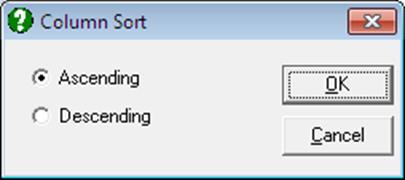
First position the active cell at any row of the column to be sorted. Then select Data → Column Sort. A dialogue will appear, giving the choice of Ascending or Descending sorts.

String variables can be selected and will be sorted according to their alphabetical ordering. Date and time variables are sorted according to their chronological order.

If the column contains missing values, they will be treated just like any other number. That is, if the missing value code is a very large negative number as suggested in Tools → Options → Memory Management, in ascending sort all missing values will move to the top of the column and in descending sort they will move to the bottom of the column.

WARNING! The Column Sort procedure sorts a column in its own place. If you need a copy of the unsorted form of the column, then you must save or copy it beforehand.

An alternative way of sorting a column is using the function Sort(Cn) (see 3.4.2.5. Statistical Functions).

3.3.4. Key Sort

The standard variable selection dialogue will allow you to select the key columns by clicking on [Variable]. When the selection process is complete click on [Finish] to perform the sort.

WARNING! The Key Sort procedure sorts the selected columns in their own place. If you need a copy of the unsorted form of the columns, then you must save or copy them beforehand.

String variables can be selected and will be sorted according to their alphabetical ordering. Date and time variables are sorted according to their chronological order.

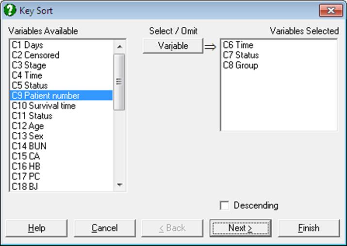
The Key Sort will sort the first column in the right list first, keeping the relative row positions of all other marked columns. If the first column contains groups of equal values then Key Sort will proceed to the second column selected and sort recursively only those groups of numbers which correspond to the equal value groups of the first column. This process is repeated until all choice columns are sorted.

In most cases, all columns involved in Key Sort will be of the same length. In the unlikely event of the marked columns having unequal lengths, Key Sort will consider empty cells of all columns below the maximum column length as missing and proceed with sorting. As in the case of single Column Sort, missing values are treated like ordinary numbers.

3.3.5. Matrix Sort

This procedure will sort the rows of the data matrix according to a single key column, keeping the rows themselves intact.

Place the active cell on the key column first and then select Data → Matrix Sort. A dialogue box, similar to the one in Column Sort procedure, will offer a choice of Ascending or Descending sorts. All rows of the data matrix will be sorted according to this column.

WARNING! The Matrix Sort procedure sorts the selected columns in their own place. If you need a copy of the unsorted form of the columns, then you must save or copy them beforehand.

3.3.6. Recode Column

This procedure is used to assign new values to the specified value ranges of a range of columns. First highlight the range of columns to recode. Non contiguous blocks of columns can be selected by pressing [Ctrl] first. After selecting Data → Recode Column a dialogue will be displayed.

All types of data (numeric, string, date and time) can be recoded. The program will select editing fields according to the type of the variable selected.

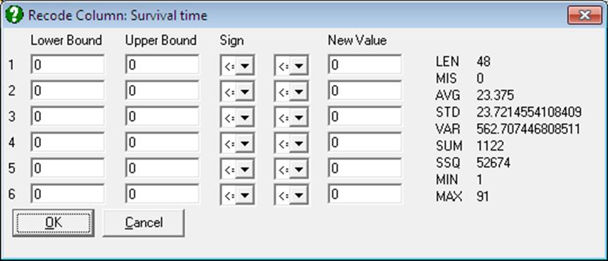
Each row of the dialogue allows for entering information about a particular interval. The first field is for the lower bound and the second is for the upper bound of the interval. The next two controls are drop-down lists for the signs of the lower and upper bounds (lb and ub). The default values of these signs are both ≤. The possible combinations are:

1)    lb ≤ x < ub,

2)    lb ≤ x ≤ ub,

3)    lb < x ≤ ub and

4)    lb < x < ub.

The last text field is for the new value of the interval. This can be an asterisk (*) for missing values.

Any row that displays a valid interval (i.e. lb ≤ ub) will be recoded. Therefore, any row left with lb = 0 and ub = 0 values (or for a string variable lb and ub left empty) will remain inactive. Information about the first column of the range to recode is displayed on the right of the screen to help with the process of entering interval limits.

WARNING! The Recode procedure changes the values of a column in their own place. If you need a copy of the original form of the column, then you must save or copy it beforehand.

Up to six intervals can be specified at a time. Note, however, that since the intervals not recoded will retain their original values, the Data → Recode Column procedure can be run more than once on the same range of columns.

3.3.7. Aggregate

Data sets with a large number of rows can be compressed for further processing. A row-wise compression is made according to the levels of a factor column. One of the following ten Scalar Functions can be used for end values: Len(), Mis(), Avg(), Var(), Std(), Ser(), Sum(), Ssq(), Min() and Max().

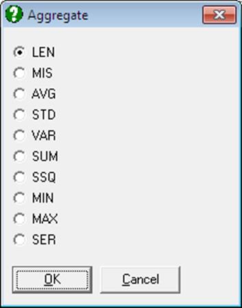
The way this procedure works is similar to that of the Matrix Sort procedure. First, move the active cell to a factor column. A factor column can be a character or numeric data column and should have a limited number of distinct values. Then select Data → Aggregate and select the function to be used in compression. First a Matrix Sort is performed. Then rows of the matrix corresponding to each distinct value of the factor column are collapsed into a single row, using the scalar function selected. For instance, if Avg() is selected then the arithmetic mean of the original rows corresponding to the same factor value will constitute a single row of the new matrix.

Columns containing non numeric data cannot be aggregated by taking their average, sum, etc. They can be aggregated only when one of the following functions is selected: Len(), Mis(), Min() and Max(). The first two functions will convert the column into a numeric column. If any other function is used the resultant column will be filled with missing values.

3.3.8. Range Statistics

It is possible to highlight a block of cells, generate row-wise or column-wise summary statistics and place the results in a column or row of the spreadsheet. The following options are offered:

1)    Column statistics into a column

2)    Column statistics into a row

3)    Row statistics into a column

4)    Row statistics into a row

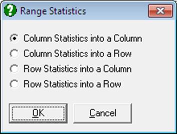
The selected statistic can be one of the ten Scalar Functions, i.e., Len(), Mis(), Avg(), Var(), Std(), Ser(), Sum(), Ssq(), Min() and Max().

First, highlight a block of cells and select Data → Range Statistics, then select one of the four options mentioned above. Then move the active cell to the start of the destination range and press <Enter/OK>. A dialogue will appear allowing you to choose from these ten statistics.

The procedure will not terminate after entering a single statistic. Assuming you will want to get more than one statistic on the same block of cells, it will work in a circular fashion. Immediately after selecting a statistic from the dialogue, you can move the active cell to a different position and press <Enter/OK> again. The Range Statistics dialogue will appear again, allowing you to select a different statistic. To break out of the loop, press <Escape/Cancel>.

3.3.9. Stack Columns

Data → Stack Columns and the accompanying Data → Unstack Columns are highly specialised but powerful procedures. The Stack Columns procedure is used to stack a number of blocks of data columns. An extra (factor) column will be created which keeps track of the blocks stacked together.

The Stack Columns procedure is particularly useful if there is data on different subjects and / or treatments and it is decided to perform Analysis of Variance. Because the Analysis of Variance procedure requires a factor column to indicate the levels of treatment for a dependent variable, the user is often faced with the cumbersome task of editing data files into this format. Stack Columns will automatically arrange data suitable for various procedures that require factor columns, such as Analysis of Variance, Break-Down, Table of Means or some nonparametric tests.

First highlight the range of columns to be stacked, then select Data → Stack Columns.

WARNING! The Stack procedure cannot be used unless a column or a range of columns has been highlighted first.

The program will ask for the number of columns per block. Since blocks of columns (i.e. not only single columns) can be stacked together, you must specify the number of columns per block. If only single columns are to be stacked, then accept the program’s choice 1 by pressing <Enter/OK>. Otherwise enter your own choice. The total number of highlighted columns must be divisible by the number of columns per block. If this condition is not met, then the program will repeat the number of columns input until a valid number is entered or <Escape/Cancel> is pressed.

Then, move the active cell to the desired location and press <Enter/OK>. An extra column containing factor levels (i.e. the number of source blocks) will be added to the front of the stacked block of columns. The length of the stacked column block will be equal to the sum total of lengths of all blocks. With large data sets, this may exceed the number of rows available in the Data Processor. If such is the case, save your data first, increase the number of rows from Tools → Options → Memory Management, load back the data and then perform the Stack Columns procedure.

3.3.10. Unstack Columns

This is the reverse of Stack Columns procedure. A block of columns will be divided into separate blocks according to the groups of similar values in the first column of the source block. Therefore, the first column of the block is expected to be a factor column with a limited number of levels (i.e. distinct values). Factor levels can be any floating point numbers, string, date or time data and they need not be sorted. The Unstack Columns procedure will first sort the block according to the (first) factor column and then create a new block for each distinct value of the factor column. Missing values are treated like ordinary numbers and a separate block is created for them.

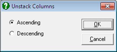
First highlight the range of columns to be unstacked, then select Data → Unstack Columns.

WARNING! The Unstack Columns procedure cannot be used unless a range of columns, the first of which is a factor column, has been highlighted first.

A dialogue will offer a choice of Ascending or Descending sorts. If the lengths of columns in the highlighted range are not equal, shorter columns will be padded up with missing values.

WARNING! The Unstack Columns procedure will sort the source columns in their own places. If you need a copy of the original form of the columns, then you must save or copy them beforehand.

The number of columns generated is directly proportional to the number of levels of the factor column and this can be substantial even with moderately large data sets. If this number exceeds the number of columns available in the Data Processor, then save your data first, increase the number of columns from Tools → Options → Memory Management, load back the data and then perform the Unstack Columns procedure.

3.3.11. Format Columns

It is possible to display all numbers in a range of columns in a specified format (e.g. decimal, exponential, integer) such that all decimal points (if there are any) are displayed at a fixed position.

All format types will affect only the display of numbers but not their significant digits in memory. To change the actual numbers use the Round() function (see 3.4.2.5. Statistical Functions).

WARNING! The format procedure cannot be used unless a column or range of columns has been highlighted first.

Highlight the range of columns to be formatted first and then select Data → Format Columns. A dialogue will appear providing access to the following format options.

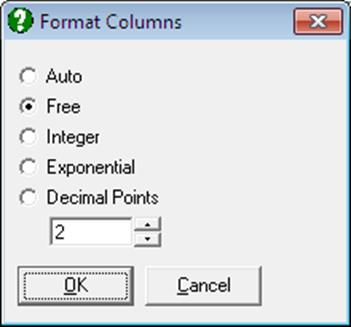
Auto: This will display as many significant digits as possible, at the same time maintaining a fixed position for the decimal point. If this cannot be done, i.e. if the column contains too small and too large numbers which are not exponential, then all numbers will be displayed in free format (see the next paragraph). If there is at least one exponential number in the column then the format will be exponential.

Free: This will in effect undo all other format types and revert to the unformatted display of numbers. This means that no zeros after the last significant digit are displayed, only too small or too large numbers are displayed in exponential format and thus decimal points are not necessarily lined up at a fixed position.

      When fresh data is entered in a column which was previously formatted, then the initial format will be retained. In this case you can reformat the column selecting one of Auto or Free options.

Integer: No floating points are displayed. Decimal numbers are rounded to the nearest integer.

Exponential: One digit will be displayed before the floating point, and two digits after it. This is followed by E, the sign of the power term (- or +) and then the power term (maximum three digits).

Decimal Points: You can choose the number of digits to be displayed after the floating point. However, the maximum number of digits to be displayed depends on the largest positive or the smallest negative number in the column. If the choice is unacceptable, then a message will be issued.

3.3.12. Select Row

This menu item is used to mark a column containing categorical data as a row-wise selection criterion for the subsample of rows (cases) to include in all subsequent analyses. This functionality is also known as select-if. You can enter a logical condition (an If() function) to fill a new column with True and False values. In all subsequent graphical or statistical procedures, only those rows that contain a True value will be included in the analysis. UNISTAT considers the value 0 as False and any other value as True.

Once a column is selected using this option, it will remain active until another column is selected by Select Row or it is deleted. To deselect a Select Row column without deleting it, place the active cell on this column and select Data → Select Row once again. Alternatively, you can also use the Data Processor’s Select function to select and deselect a Select Row column (see 3.4.2.6.3. UNISTAT Functions). At any one time, there can only be one Select Row column in the Data Processor. The colour of the Select Row column can be changed from Tools → Options → Colours.

A Select Row column may be generated by the program automatically when outliers are deleted from a regression graph (see 2.3.2.3. Interactive Data Points), or a rectangular block of cells is highlighted in Data Processor before selecting a procedure.

In Excel Add-In Mode, when a Select Row column is created automatically by deleting outliers from a regression graph interactively, the only way to switch it off is to highlight a different block of data in Excel.